Linear Filters: Image Filtering & Modification

1. Linear filters

2. What is Image Filtering? Modify the pixels in an image based on some function of a local neighborhood of the pixels Some function University of Missouri at Columbia

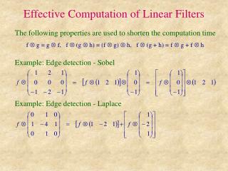
3. Linear Filtering • Linear case is simplest and most useful • Replace each pixel with a linear combination of its neighbors. • The prescription for the linear combination is called the convolution kernel. kernel University of Missouri at Columbia

4. f(.) f(.) f(.) f(.) f(.) f(.) f(.) f(.) f(.) c11 c12 c13 c23 c21 c22 c31 c32 c33 +c12f(i-1,j) +c13f(i-1,j+1) + c11f(i-1,j-1) + c22f(i,j) + c23f(i,j+1) + c21f(i,j-1) + c33f(i+1,j+1) c31f(i+1,j-1) + c32f(i+1,j) Convolution o (i,j) =  University of Missouri at Columbia

5. Linear Filter = Convolution University of Missouri at Columbia

6. Filtering Examples University of Missouri at Columbia

7. Filtering Examples University of Missouri at Columbia

8. Filtering Examples University of Missouri at Columbia

9. Averaging Gaussian Smoothing With Gaussian University of Missouri at Columbia

10. General process: Form new image whose pixels are a weighted sum of original pixel values, using the same set of weights at each point. Properties Output is a linear function of the input Output is a shift-invariant function of the input (i.e. shift the input image two pixels to the left, the output is shifted two pixels to the left) Example: smoothing by averaging form the average of pixels in a neighbourhood Example: smoothing with a Gaussian form a weighted average of pixels in a neighbourhood Example: finding a derivative form a weighted average of pixels in a neighbourhood Linear Filters University of Missouri at Columbia

11. Represent these weights as an image, H H is usually called the kernel Operation is called convolution it’s associative Convolution • Result is: • Notice wierd order of indices • all examples can be put in this form • it’s a result of the derivation expressing any shift-invariant linear operator as a convolution. University of Missouri at Columbia

12. Example: Smoothing by Averaging University of Missouri at Columbia

13. Smoothing with an average actually doesn’t compare at all well with a defocussed lens Most obvious difference is that a single point of light viewed in a defocussed lens looks like a fuzzy blob; but the averaging process would give a little square. A Gaussian gives a good model of a fuzzy blob Smoothing with a Gaussian University of Missouri at Columbia

14. The picture shows a smoothing kernel proportional to (which is a reasonable model of a circularly symmetric fuzzy blob) An Isotropic Gaussian University of Missouri at Columbia

15. Recall Now this is linear and shift invariant, so must be the result of a convolution. We could approximate this as (which is obviously a convolution; it’s not a very good way to do things, as we shall see) Differentiation and convolution University of Missouri at Columbia

16. Finite differences University of Missouri at Columbia

17. Simplest noise model independent stationary additive Gaussian noise the noise value at each pixel is given by an independent draw from the same normal probability distribution Issues this model allows noise values that could be greater than maximum camera output or less than zero for small standard deviations, this isn’t too much of a problem - it’s a fairly good model independence may not be justified (e.g. damage to lens) may not be stationary (e.g. thermal gradients in the ccd) Noise University of Missouri at Columbia

18. sigma=1 University of Missouri at Columbia

19. sigma=16 University of Missouri at Columbia

20. Finite difference filters respond strongly to noise obvious reason: image noise results in pixels that look very different from their neighbours Generally, the larger the noise the stronger the response What is to be done? intuitively, most pixels in images look quite a lot like their neighbours this is true even at an edge; along the edge they’re similar, across the edge they’re not suggests that smoothing the image should help, by forcing pixels different to their neighbours (=noise pixels?) to look more like neighbours Finite differences and noise University of Missouri at Columbia

21. Finite differences responding to noise Increasing noise -> (this is zero mean additive gaussian noise) University of Missouri at Columbia

22. Do only stationary independent additive Gaussian noise with zero mean (non-zero mean is easily dealt with) Mean: output is a weighted sum of inputs so we want mean of a weighted sum of zero mean normal random variables must be zero Variance: recall variance of a sum of random variables is sum of their variances variance of constant times random variable is constant^2 times variance then if s is noise variance and kernel is K, variance of response is The response of a linear filter to noise University of Missouri at Columbia

23. Filter responses are correlated • over scales similar to the scale of the filter • Filtered noise is sometimes useful • looks like some natural textures, can be used to simulate fire, etc. University of Missouri at Columbia

24. University of Missouri at Columbia

25. University of Missouri at Columbia

26. University of Missouri at Columbia

27. Generally expect pixels to “be like” their neighbours surfaces turn slowly relatively few reflectance changes Generally expect noise processes to be independent from pixel to pixel Implies that smoothing suppresses noise, for appropriate noise models Scale the parameter in the symmetric Gaussian as this parameter goes up, more pixels are involved in the average and the image gets more blurred and noise is more effectively suppressed Smoothing reduces noise University of Missouri at Columbia

28. The effects of smoothing Each row shows smoothing with gaussians of different width; each column shows different realisations of an image of gaussian noise. University of Missouri at Columbia

29. Some other useful filtering techniques • Median filter • Anisotropic diffusion University of Missouri at Columbia

30. Median filters : principle • non-linear filter • method : • 1. rank-order neighbourhood intensities • 2. take middle value • no new grey levels emerge... University of Missouri at Columbia

31. Median filters : odd-man-out advantage of this type of filter is its “odd-man-out” effect e.g. 1,1,1,7,1,1,1,1  ?,1,1,1.1,1,1,? University of Missouri at Columbia

32. Median filters : example filters have width 5 :  University of Missouri at Columbia

33. Median filters : analysis median completely discards the spike, linear filter always responds to all aspects median filter preserves discontinuities, linear filter produces rounding-off effects DON’T become all too optimistic  University of Missouri at Columbia

34. 3 x 3 median filter : sharpens edges, destroys edge cusps and protrusions Median filter : images  University of Missouri at Columbia

35. Median filters : Gauss revisited Comparison with Gaussian : 3 x 3 median filter : sharpens edges, destroys edge cusps and protrusions e.g. upper lip smoother, eye better preserved  University of Missouri at Columbia

36. Example of median 10 times 3 X 3 median patchy effect important details lost (e.g. ear-ring)  University of Missouri at Columbia

37. Pyramids

38. Linear filters Gaussian blurring Finite differences Composition of linear filters = linear filter Corners, etc. Edge detection University of Missouri at Columbia

39. Big bars (resp. spots, hands, etc.) and little bars are both interesting Stripes and hairs, say Inefficient to detect big bars with big filters And there is superfluous detail in the filter kernel Alternative: Apply filters of fixed size to images of different sizes Typically, a collection of images whose edge length changes by a factor of 2 (or root 2) This is a pyramid (or Gaussian pyramid) by visual analogy Scaled representations University of Missouri at Columbia

40. A bar in the big images is a hair on the zebra’s nose; in smaller images, a stripe; in the smallest, the animal’s nose University of Missouri at Columbia

41. Aliasing • Can’t shrink an image by taking every second pixel • If we do, characteristic errors appear • In the next few slides • Typically, small phenomena look bigger; fast phenomena can look slower • Common phenomenon • Wagon wheels rolling the wrong way in movies • Checkerboards misrepresented in ray tracing • Striped shirts look funny on colour television University of Missouri at Columbia

42. Resample the checkerboard by taking one sample at each circle. In the case of the top left board, new representation is reasonable. Top right also yields a reasonable representation. Bottom left is all black (dubious) and bottom right has checks that are too big. University of Missouri at Columbia

43. Constructing a pyramid by taking every second pixel leads to layers that badly misrepresent the top layer University of Missouri at Columbia

44. Open questions • What causes the tendency of differentiation to emphasize noise? • In what precise respects are discrete images different from continuous images? • How do we avoid aliasing? • General thread: a language for fast changes The Fourier Transform University of Missouri at Columbia

45. Represent function on a new basis Think of functions as vectors, with many components We now apply a linear transformation to transform the basis dot product with each basis element In the expression, u and v select the basis element, so a function of x and y becomes a function of u and v basis elements have the form The Fourier Transform transformedimage vectorized image Fourier transform base,. University of Missouri at Columbia

46. To get some sense of what basis elements look like, we plot a basis element --- or rather, its real part --- as a function of x,y for some fixed u, v. We get a function that is constant when (ux+vy) is constant. The magnitude of the vector (u, v) gives a frequency, and its direction gives an orientation. The function is a sinusoid with this frequency along the direction, and constant perpendicular to the direction. University of Missouri at Columbia

47. Fourier basis element • example, real part • Fu,v(x,y) • Fu,v(x,y)=const. for (ux+vy)=const. • Vector (u,v) • Magnitude gives frequency • Direction gives orientation. University of Missouri at Columbia

48. Here u and v are larger than in the previous slide. University of Missouri at Columbia

49. And larger still... University of Missouri at Columbia

50. Fourier transform of a real function is complex difficult to plot, visualize instead, we can think of the phase and magnitude of the transform Phase is the phase of the complex transform Magnitude is the magnitude of the complex transform Curious fact all natural images have about the same magnitude transform hence, phase seems to matter, but magnitude largely doesn’t Demonstration Take two pictures, swap the phase transforms, compute the inverse - what does the result look like? Phase and Magnitude University of Missouri at Columbia