Download
1 / 88
880 likes | 885 Vues
This article discusses the importance of studying the ionosphere and the challenges associated with accurate monitoring and forecasting of ionospheric disturbances. It highlights how GPS can contribute to near real-time, high-resolution, global total electron content (TEC) estimates.

E N D
Part II MAPPING THE IONOSPHERE WITH GPS GS894G
References Wielgosz, P. The impact of ionospheric effects on GPS data reduction, PhD dissertation, UWM, Poland, 2002 (in Polish)Bosy, J, M. Figurski, P. Wielgosz. The strategy of GPS data processing in precise local networks during high solar activity, GPS Solutions, 2003 (in print)Schaer, S. Mapping and Predicting the Earth's Ionosphere Using the Global Positioning System, PhD thesis, University of Bern, 1999. Ron Muellerschoen, R. and Powers, E. Errors in GPS due to Satellite C1- P1 Code Biases Hajj, G. A. et al. (2000): COSMIC GPS Ionospheric Sensing and Space Weather, TAO, Vol. 11, No. 1, pp. 235-272.http://www.spaceweather.com/ http://www.ips.gov.au/Main.php?CatID=8 http://nssdc.gsfc.nasa.gov/space/model/models_home.html http://www.cx.unibe.ch/aiub/ionosphere.html http://www.sunspotcycle.com/
Introduction to the ionosphere • The ionosphere is the part of the upper atmosphere where free electrons occur in sufficient density to have a substantial influence on the propagation of radio frequency electromagnetic waves (such as GPS) • The ionization depends primarily on the solar activity • Ionospheric structures and peak densities in the ionosphere vary greatly with time and location, and thus, must be monitored
Why do we need to study ionosphere? • The spatial and temporal distributions of ionospheric disturbances, such as storms and Traveling Ionospheric Disturbances (TIDs), are of primary interest in their own scientific context, but they are also of special interest to communication, surveillance and radio-navigation, since they affect the skywave signal channel characteristics. • Thus, the communication and navigation systems (GPS) relying on trans-ionospheric propagation must be able to account for the effects of the abrupt changes in total electron content (TEC), associated with the storm time disturbance effects, including the occurrence of the ionospheric trough at mid-latitudes. • Conversely: if the GPS receiver’s location is known, GPS observable may allow to track ionospheric properties
Why do we need to study ionosphere? • As our dependence on technology in space grows, continuous and global sensing of the Earth’s atmosphere is becoming a technological necessity. • The awareness of the potentially hazardous effects of space weather on technological systems motivated the creation of the National Space Weather Program (NSWP) • NSWP places particular emphasis on the need to provide timely, accurate, and reliable space environment observations, specifications, and forecasts • These requirements are similar to what is already accomplished with a great measure of success in the Numerical Weather Prediction (NWP) – currently exclusively relying on remote sensing techniques.
Currentchallenges • Accurate specification and forecasting of space weather phenomena is very difficult because it requires: • accurate modeling of the coupling between the sun, the magnetosphere, the thermosphere, the ionosphere, and the mesosphere, • continuous, reliable and accurate observations of all of these regions • the ability to assimilate the data into the models in an optimal and self-consistent manner. GPS can contribute greatly by providing near real-time, high resolution, global TEC estimates
Ionization is caused by: • X-ray radiation • ultraviolet radiation • corpuscular radiation from the Sun • Ionospheric structures and peak densities vary with: • time (sunspot cycle, season, local time, i.e., day vs. night) • geographic location (polar, auroral zones, mid-latitudes (lowest ionospheric variability), and equatorial regions (the largest electron content)) • certain solar-related ionospheric disturbances • The motion and distribution of the electrons is affected by Earth magnetic field • Electrons move along magnetic lines of force • Thus, electron distribution is described in terms of geomagnetic coordinates • north geomagnetic pole: 79.41 and –71.64 (epoch 1998.5) slowly moving (0.03 and 0.07 per year)
Solar – Earth connection Influence of the solar wind on earth’s magnetosphere
Why do we need to study ionosphere? • Peak values of electron density are encountered in the equatorial region, normally in the early afternoon • Region with very high electron concentration at geomagnetic latitudes of about +/- 20 deg during early evening (maxima are referred to as equatorial anomaly) • The mid-latitude ionosphere shows the least variations. It is also best observed as most of the ionosphere sensing instruments are located in this region. • In the high latitudes and auroral zones the peak electron densities are smaller than in lower latitudes. However, this sector is extremely rich in plasma instabilities, which implies that short-term variations in the electron density are more pronounced there than at lower latitudes • At polar caps, where the solar zenith angle is essentially constant, a diurnal variation is still detectable, indicating that apart from solar illumination there are other factors that affect the state of the ionosphere
Global TEC map at 14:30 UT September 11, 1994. Clearly visible equatorial anomaly (National Space Science Data Center)
Why do we need to study ionosphere: ionospheric irregularities • significant variations in electron density are caused by traveling ionospheric disturbances (TIDs) • large-scale TIDs, periods of 30 min to 3 hours, and horizontal wavelengths exceeding 1000 km • medium-scale TIDs, periods from 10 min to 1 hour, and horizontal wavelength of several hundreds of km • small-scale TIDs, periods of several minutes, and horizontal wavelength of tens of km • smallest-scale structures in the electron density distribution cause scintillation1 effects, rapid variations in the line-of-sight electron content (equatorial, high-latitude and polar regions) • ionospheric storms: vast and massive ionospheric events, often coupled with severe disturbances in the magnetic field and intense solar eruptions (flares) • usually results in a tremendous increase of electron content
Vertical electron distribution • Vertical regions • Peak density in F region • Different distribution • during day and night Ne-
Vertical electron distribution • Region F starts at ~150 km • Consists of F1 and F2 • formed primarily due to ultraviolet radiation • Regions E and D are due to X-ray radiation • Effect of D on GPS signal propagation are negligible • F1 combined with E effects accounts for 10% of GPS ionospheric delay • F2 has the highest electron concentration (250-450 km) and largest variability, and accounts for up to 80% of GPS ionospheric delay • Upper boundary of ionosphere is not clearly defined, however, above 1000 km the electron density is very low • The ionospheric delay caused by the layer above 1000 km amounts to about 10% of the total effect during the day and ~50% during the nigh
Sunspots (February 2000) The Sun - The dark areas are the sunspots
SSN - Sunspot Number SSN=10g+s, where: g – number of groups of sunspots, s – number of individual spots.
Current cycle of solar activity SSN year
Solar events CME (Coronal Mass Ejection) Solar flare
Indices of geomagnetic activity Kp 0o 0+ 1- 1o 1+ 2- 2o 2+ 3- 3o 3+ 4- 4o 4+ ap 0 2 3 4 5 6 7 9 12 15 18 22 27 32 Kp 5- 5o 5+ 6- 6o 6+ 7- 7o 7+ 8- 8o 8+ 9- 9o ap 39 48 56 67 80 94 111 132 154 179 207 236 300 400 Kp and ap are derived every 3 hours from magnetometric observations Kp 4 - quiet magnetosphere Kp = 4 - active magnetosphere Kp = 5 - minor storm Kp 6 - major storm
Wave propagation in the ionosphere The refractive index - n describes the wave propagation in given medium. Where: c – the speed of the light in the vacuum v - the speed of the light in the medium nion > 1 for code GPS observable (code delay) nion < 1 for phase GPS observable (phase advance)
The refractive index nion can be expandedin the reciprocal frequency f of the electromagnetic wave as: With the constants: Where: Ne– electron density, H0– magnetic field strength, – angle between the propagation direction of the electromagnetic waveand the vector of the geomagnetic field, e– charge of one electron, 0– electric permittivity1 in the vacuum, me – mass of electron, 0– magnetic permeability2 in the vacuum.
Approximated values of the terms in equation below: 2nd = 210-4- delay/advance (we account for this part only) 3rd = 210-7- bending (neglected in the ion computation) 4th = 210-8- different ray paths (neglected in the ion computation)
the signal delay depends on the total electron content (TEC) along the signal’s path and on the frequency of the signal itself as well as on the geographic location and time and solar activity, as explained earlier • integration of the refractive index renders the measured range, and the ionospheric terms for range and phase are as follows: • TEC is the line-of-sight TEC in electrons per square meter. Usually expressed in TECU (TEC Units), where one TECU corresponds to 1016 electrons contained in a cylinder aligned along the line of sight with a cross-section of one square meter, so 1 TECU = 1016 el/m2
Wave propagation in the ionosphere ion – path delay due to the ionosphere Cx/2 40.3 m3s-2 (40.3 1016 ms-2 TECU-1) – constant corresponding to the square of the plasma frequency divided by the electron density ( = e2/(420m ) = 40.3 Neis the electron density (number of electrons per cubic meter) along the signal’s path Naturally, if ion is known, TEC value can be estimated
Integrated electron density • For the propagation of microwaves through the ionosphere • the electron density integrated along the ray path, generally called • TEC (Total Electron Content), is the important ionospheric quantity • Neis the electron density (number of electrons per cubic meter) • along the signal’s path • The term TEC is often used to designate the VTEC (Vertical TEC) • – slant TEC reduced to the vertical using mapping function F(z), which is a ratio of slant TEC to VTEC
SLM – Single Layer Model z’ is elevation angle at ionosphere piercing point SLM assumes that all free electrons are contained in a shell of infinitesimal thickness at altitude H
Linear combination path delay / 1 TECU m cycles L1 L2 L3 (iono. Free) L4(geo. free) L5(wide-lane) 0.162 0.267 0 -0.105 -0.208 0.853 1.095 0 -1.948 -0.248 Ionospheric path delay caused by 1TECU of free electrons Define a constant that gives the ionospheric path delay per TECU referred to the first GPS frequency f1 (also denoted as 1) The path delays expressed in meters per TECU are equal to Where , 4 and 5 equal to
13 UT TECU Latitude 15 UT Global TEC maps 17 UT longitude
DD residual ionospheric delay on wide-line combination for 300 km baseline Cycles L5 UT hours Processing without ionospheric information from the maps Cycles L5 UT hours Processing with ionospheric information from the maps
Negative sign implies an apparent reduction in baseline length Where lion is the iono-induced distance bias to be expected, and l is the baseline vector R is the length of the geocentric receiver vector (approximately the Earth radius) zmax is the maximum satellite zenith distance imposed in the processing
Influence of the Antarctic ionosphere on static GPS positioning: example • Data processing: • IGS observations • 24-hour sessions with 1 hour overlap • 7 deg. elevation mask • Elevation-dependent observation weighting • QIF (Quasi Ionosphere Free) ambiguity resolution
Correlation between averaged TEC over a baseline and rms of obtained ambiguities
% of resolved ambiguities Correlation between % of resolved ambiguities and obtained length of the vector % of resolved ambiguities
Ionospheric delay observed by the ground-based permanently tracking stations • almost impossible to derive height-dependent ionospheric profile • Observed GPS delay by the Low Earth Orbiter (LEO) at the instant of GPS satellite occultation by Earth limb • GPS signal bent and delay are associated with the vertical profiles of atmospheric parameters • With full GPS constellation several hundreds of daily occultations can be observed by a single LEO • A constellation of LEOs is needed for global coverage • Ionosphere tomography • Only ground-based solution is considered here
TEC estimation with GPS • Only ground-based solution is considered here • For ground-based absolute TEC mapping, the TEC along the vertical is of main interest • GPS provides in principle slant TEC, so mapping function is needed to convert it to VTEC • to refer the resulting VTEC to specific solar-geomagnetic coordinates, the single-layer (thin shell) model is usually adopted for the ionosphere • Assume that free electrons are all contained in a shell of infinitesimal thickness at altitude H (350, 400 or 450 km)
TEC estimation with GPS • Difference in ionospheric delay between the observables on L1 and L2 is used • Each 1 meter of differential delay between L1 and L2 corresponds roughly to 10 TECU1 • Geometry-free combination is most commonly used • Relative TEC – from carrier phase • Absolute TEC – from pseudorange
SLM – Single Layer Model SLM assumes that all free electrons are contained in a shell of infinitesimal thickness at altitude H
Assuming the homogeneous satellite distribution over the entire sky, the semi diameter of the ionospheric cap probed by a single receiver is defined by the maximum central angle zmax. z and z’ are zenith distance at GPS receiver and ionosphere piercing point (IPP); R is geocentric distance to the receiver and H is the assumed height of the ionospheric layer (here assumed at 450 km)
The number of stations sufficient to sound out the entire Earth ionosphere equals to: So, for zmax=80 deg, nA = ~ 80 stations The steradian (symbolized sr) is the Standard International (SI) unit of solid angular measure. There are 4 pi, or approximately 12.5664, steradians in a complete sphere. A steradian is defined as conical in shape, as shown in the illustration. Point P represents the center of the sphere. The solid (conical) angle q, representing one steradian, is such that the area A of the subtended portion of the sphere is equal to r2, where r is the radius of the sphere.
Ionospheric delay in GPS equations - satellite and receiver clock errors wrt GPS time • constant bias expressed in cycles; in principal, it contains the • initial carrier phase ambiguity; it is a real-valued number • containing the integer ambiguity, effect of phase windup1and • satellite and receiver hardware delays • satellite and receiver hardware delays in units of time; normally • ignored as they cannot be separated from the clock errors. Clock • errors compensate for hardware delays
Introducing the ionosphere variable Iik ( ),which represents the ionospheric delay related to first frequency, 1(notice that 1corresponds to our earlier notationf1)
Pseudorange smoothing Smoothed, dual frequency pseudorange at epoch t and The noise on smoothed pseudorange is reduced by sqrt(n), where n is the number of epochs used in the smoothing process; it is used in ionosphere estimation
Double difference equations Ambiguities, N, are integers, as clock errors and hardware biases were eliminated (greatly reduced) by differencing.
Geometry free linear combination (LC): of vital interest to ionosphere estimation cancels frequency independent errors In un-differenced mode
What are DCBs and what is the reason for non-zero DCBs? • P1-P2 and P1-C1 biases • must be estimated for satellites and receivers
ICD-GPS-200, Revision C, Initial Release, 10 October 1993 3.3.1.8 Signal Coherence. All transmitted signals for a particular SV shall be coherently derived from the same on-board frequency standard; all digital signals shall be clocked in coincidence with the PRN transitions for the P-signal and occur at the P-signal transition speed. On the L1 channel the data transitions of the two modulating signals (i.e., that containing the P(Y)-code and that containing the C/A-code) shall be such that the average time difference between the transitions does not exceed 10 nanoseconds (two sigma).