Download

1 / 44
440 likes | 574 Vues
Stochastic Methods. A Review. Some Terms. Random Experiment : An experiment for which the outcome cannot be predicted with certainty Each experiment ends in an outcome The collection of all outcomes is called the sample space , S An event is a subset of the sample space

E N D
Stochastic Methods A Review
Some Terms Random Experiment: An experiment for which the outcome cannot be predicted with certainty Each experiment ends in an outcome The collection of all outcomes is called the sample space, S An event is a subset of the sample space Given a random experiment with a sample space, S, a function X that assigns to each element s in S a real number, X(s) = x, is called a random variable. A boolean random variable is a function from an event to the set {false, true} (or {0.0,1.0}).
Bernoulli/Binomial Experiments • A bernoulli experiment is a random experiment the outcome of which can be classified in one of two mutually exclusive and exhaustive ways ({failure,success}, {false,true}, {0,1}), etc. • A binomial experiment is a bernoulli experiment that: • Is performed n times • The trials are independent • The probability of success on each trial is a contant, p. • The probability of failure on each trial is a constant 1 – p • A random variable counts the number of successes in n trials
Example A • A fair die is cast six times • Success: a six is rolled • Failure: all other outcomes • A possible observed sequence is (0,0,1,0): a six has been rolled on the third trial. Call this sequence A. • Since every trial in the sequence is independent, p(A) = 5/6 * 5/6 * 1/6 * 5/6 = (1/6)(5/6)3
Example A’ • Now suppose we want to know the probability of 1 six in any four roll sequence: (0001),(0010),(0100),(1000) = 4 * p(A) since there are four ways of selecting 1 position for the 1 success
In General • The number of ways of selecting y positions for y successes in n trials is: • nCy = n! /((n – y)! * y!) The probability of each of these ways is the probability of success * the probability of failure • py* (1-p)n-y • So, if Y is the event of y successes in n trials, p(Y) = nCy* py * (1-p)n-y
This is Exactly the Example • p(Y) = nCy* py * (1-p)n-y • A fair die is cast six times • Success: a six is rolled • Failure: all other outcomes • n=4 • y = 1 • 4C1 = 4!/(4-1)! * 1! = 4 • py = (1/6)1 • (1-p)4-1 = (5/6)3
What is the probability of obtaining 5 heads in 7 flips of a fair coin • The probability of the event X, p(X), is the sum of the probabilities of each individual events (nCx)px(1-p)n-x • The Event X is 5 successes out of seven tries • n = 7, x = 5 • p(of a single success) = ½ • p(of a single failure) = ½ • P(X) = (7C5)(1/2)5(1/2)2 = .164 • The tries can be represented like this: • {0011111}, {0101111} … • There are 21 of the, each with a probability of :(1/2)5(1/2)2
Expectation If the reward for the occurrence of an event E, with probability p(E), is r, and the cost of the event not occurring, 1-p(E), is c, then the expectation for an event occurring, ex(E), is ex(E) = r x p(E) + c (1-p(E))
Expectation Example • A fair roulette wheel has integers, 0 to 36. • Each player places 5 dollars on any slot. • If the wheel stops on the spot, the player wins $35, else she loses $1 • So, p(winning)= 1/37 P(losing) = 36/37 ex(E) = 35(1/37) + (-5)(36/37) ~$-3.92
Bayes Theorem For Two Events Recall that we defined conditional probability like this: We can also express s in terms of d: Multiplying (2) by p(d) we get: Substituting (3) into (1) gives Bayes’ theorem for two events 1 2 3
If d is a disease and s is a symptom, the theorem tells us that the probability of the disease given the symptom is the probability of the symptom given the disease times the probability of the disease divided by the probability of the symptom
The Chain Rule ) = Since set intersection is commutative ) = then = Can be generalize for any N sets and proved by induction
Example Threecards are to be dealt one after another at random and without replacement from a fair deck. What is the probability of receiving a spade, a heart, a diamondin that order A1= event of being dealt a spade A2= event of being dealt a heart A3 = event of being dealt a diamond Total Probability = 13/52*13/51*13/50
An Application • Def: A probabilistic finite state machine is a finite state machine where each arc is associated with a probability, indicating how likely that path is to be taken. The sum of the probabilities of all arcs leaving a node must sum to 1.0. • A PFSM is an acceptor when one or more states are indicated as the start states and one or more states is indicated as the accept state.
Phones/Phonemes • Def: A phone is a speech sound • Def: A phoneme is a collection of related phones (allophones) that are pronounced differently in different contexts • So [t] is phoneme. • The [t] sound in tunafish differs from the [t] sound in starfish. The first [t] is aspirated, meaning the vocal chords briefly don’t vibrate, producing a sound like a puff a air. A [t] followed by an [s] is unaspirated • FSA showing the probabilities of allophones in the word “tomato”
More Phonemes • This happens with a [k] and [g]—both are unaspirated, leading to the mishearing of the Jimi Hendrix song: • ‘Scuse me, while I kiss the sky • ‘Scuse me, while I kiss this guy
Phoneme Recognition Problem • Computational Linguists have collections of spoken and written language called corpora. • The Brown Corpus and the Switchboard Corpus are two examples. Together, they contain 2.5 million written and spoken words that we can use as a base
Now Suppose • Our machine identified the phone I • Next the machine has identified the phone ni (as in “knee”) • Turns out that an investigation of the Switchboard corpus shows 7 words that can be pronounced ni after I • the,neat, need, new, knee, to, you
How can this be? • Phoneme [t] is often deleted at the end of the word: say “neat little” quickly • [the] can be pronounced like [ni] after in or. Talk like Jersey gangster here or Bob Marley
Strategy • Compile the probabilities of each of the candidate words from the corpora • Applies Baye’s theorem for two events:
Word Frequency Probability knee 61 .000024 the 114834 .046 neat 338 .00013 need 1417 .00056 new 2625 .001
Apply Simplified Bayes Since all of the candidtates will be divided by p[ni], we can drop it off giving:p(word|[ni]) p([ni]|word)p(word)) • But where does p([ni]|word) come from? • Rules of pronunciation variation in English are well-known. • Run them through the corpora and generate probabilities for each. • So, for example, that word initial [th] becomes [n] if the preceding word ended in [n] is .15 • This can be done for other pronunciation rules
Result Word p([ni]|word) p(word) p([ni]|word)p(word) New .36 .001 .00036 Neat .52 .00013 .000068 Need .11 .00056 .000062 Knee 1.0 .000024 .000024 The 0.0 .046 0.0 The has a probability of 0.0 since the previous phone was [the] not [n] Notice that new seems to be the most likely candidate. This might be resolved at the syntactic level Another possibility is to look at the probability of two word combinations in the corpora: “I new” is less probable than “I need” This is referred to as N-Gram analysis
General Bayes Theorem Recall Bayes Theorem for two events: P(A|B) = p(B|A)p(A)/p(B) We would like to generalize this to multiple events
Example Suppose: Bowl A contains 2 red and 4 white chips Bowl B contains 1 red and 2 white chips Bowl C contains 5 red and 4 white chips We want to select the bowls and compute the p of drawing a red chip Suppose further P(A) = 1/3 P(B) = 1/6 P(C) = ½ Where A,B,C are the events that A,B,C are chosen
P(R) is dependent upon two probabilities: p(which bowl) then the p(drawing a red chip) So, p(R) is the union of the probability of mutually exclusive events:
Now suppose that the outcome of the experiment is a red chip, but we don’t know which bowl it was drawn from. So we can compute the conditional probability for each of the bowls. From the definition of conditional probability and the result above, we know:
We can do the same thing for the other bowls: p(B|R) = 1/8 P(C|R) = 5/8 This accords with intuition. The probability that the red bowl was chosen increases over the original probability, because since it has more red chips, it is the more likely candidate. The original probabilities are called prior probabilities The conditional probabilities (e.g., p(A|R)) are called the posterior probabilities.
To Generalize Let events B1,B2,…,Bm constitute a partition of the sample space S. That is: Suppose R is an event with B1 …Bm its prior probabilities, all of which > 0, then R is the union m mutually exclusive events, namely,
Now, If p(A) > 0, we have from the definition of conditional probability that P(Bk|R) is the posterior probability
Example Machines A,B,C produce bolts of the same size. Each machine produces as follows: • Machine A = 35%, with 2% defective • Machine B =25%, with 1% defective • Machine C =40% with 3% defective Suppose we select one bolt at the end of the day. The probability that it is defective is:
Now suppose the selected bolt is defective. The probability that it was produced by machine 3 is: Notice how the posterior probability increased, once we concentrated on C since C produces both more bolts and a more defective bolts.
Evidence and Hypotheses We can think of these various events as evidence (E) and hypotheses (H). Where p(Hk|E) is the probability that hypothesis i is true given the evidence, E p(Hk) is the probability that hypothesis I is true overall p(E|Hk) is the probability of observing evidence, E, when Hi is true m is the number of hypotheses
Why Bayes Works The probability of evidence given hypotheses is often easier to determine than the probability of hypotheses given the evidence. Suppose the evidence is a headache. The hypothesis is meningitis. It is easier to determine the number of patients who have headaches given that they have meningitis than it is to determine the number of patients who have meningitis, given that that they have headaches. Because the population of headache sufferers is
But There Are Issues When we thought about bowls (hypotheses) and chips (evidence), the probability of a kind of bowl given a red chip required that we compute 3 posterior probabilities for each of three bowls. If we also worked it out for white chips, we would have to compute 3X2 = 6 posterior probabilities. Now suppose our hypotheses are drawn from the set of m diseases and our evidence from the set of n symptoms, we have to compute mXn posterior probabilities.
But There’s More Bayes assumes that the hypothesis partitions the set of evidence into disjoint sets. This is fine with bolts and machines or red chips and bowls, but much less fine with natural phenomena. Pneumonia and strep probably doesn’t partition the set of fever sufferers (since they could overlap)
That is We have to use a form of Bayes theorem that that considers any single hypothesis, hi, in the context of the union of multiple symptoms ei If n is the number of symptoms and m the number of diseases, this works out to be mxn2 + n2+ m pieces of information to collect. In a expert system that is to classify 200 diseases using 2000 symptoms, this is 800,000,000 pieces of information to collect.
Naïve Bayes to the Rescue • Naive Bayes classification assumes that variables are independent. • The probability that a fruit is an apple, given that it is red, round, and firm, can be calculated from the independent probabilities that the observed fruit is red, that it is round, and that it is firm. • The probability that a person has strep, given that he has a fever, and a sore throat, can be calculated from the independent probabilities that a person has a fever and has a sore throat.
In effect, we want to calculate this: Since the intersection of sets is a set, Bayes lets us write: Since we only want to classify and the denominator is constant, we can ignore it giving:
Independent Events to the Rescue Assume that all pieces of evidence are independent given a particular hypothesis. Recall the chain rule: Since p(B|A) = p(B) and p(C)|A B) = p(C), that is, the events are mutually exclusive, then
Becomes (with a little hand-waving) P(hi|E) p(e1|h)Xp(e2|hiX…Xp(en|hi)