Download
1 / 29
300 likes | 499 Vues
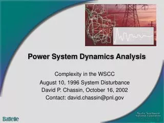
Power System Dynamics -- Postgraduate Course of Tsinghua Univ. Graduate School at Shenzhen. NI Yixin Associate Professor Dept. of EEE, HKU <yxni@eee.hku.hk>. Introduction. 0.1 Requirements of modern power systems (P. S. ) 0.2 Recent trends of P. S. 0.3 Complexity of modern P. S.

E N D
Power System Dynamics-- Postgraduate Course of Tsinghua Univ. Graduate School at Shenzhen NI Yixin Associate Professor Dept. of EEE, HKU <yxni@eee.hku.hk>
Introduction 0.1 Requirements of modern power systems (P. S. ) 0.2 Recent trends of P. S. 0.3 Complexity of modern P. S. 0.4 Definitions of different types of P. S. stability 0.5 Computer-aid P. S. stability analysis 0.6 Contents of our course
Introduction (1) 0.1 Requirements of modern power systems (P. S. ) • Satisfying load demands (as a power source) • Good quality: voltage magnitude, symmetric three phase voltages, low harmonics, standard frequency etc. (as a 3-phase ac voltage source) • Economic operation • Secure and reliable operation with flexible controllability • Loss of any one element will not cause any operation limit violations (voltage, current, power, frequency, etc. ) and all demands are still satisfied. • For a set of specific large disturbances, the system will keep stable after disturbances. • Good energy management systems (EMS)
Introduction (2) 0.2 Recent trends of P. S. • Systems interconnection: to obtain more benefits. It may lead to new stability issues ( e.g. low-frequency power oscillation on the tie lines; SSR caused by series-compensated lines etc. ). • Systems are often heavily loaded and very stressed. System stability under disturbances is of great concern. • New technology applications in power systems. (e.g. computer/ modern control theory/ optimization theory/ IT/ AI tech. etc. ) • Power electronics applications: provides flexible controller in power systems. ( e. g. HVDC transmission systems, STATCOM, UPFC, TCSC, etc.)
Introduction (3) 0.3 Complexity of modern P. S. • Large scale, • Hierarchical and distributed structure, • Non-storable electric energy, • Fluctuate and random loads, • Highly nonlinear dynamic behavior, • Unforeseen emergencies, • Fast transients which may lead to system collapse in seconds or minutes, • Complicated control and their coordination requests. -- Modern P. S. is much more complicated than ever and in the meantime it plays a significant role in modern society.
Introduction (4) Some viewpoints of Dr. Kundur (author of the ref. book ): --- The complexity of power systems is continually increasing because of the growth in interconnections and use of new technologies. At the same time, financial and regulatory constrains have forced utilities to operate the systems nearly at stability limits. --- Of all the complex phenomena on power systems, power system stability is the most intricate to understand and challenging to analyze. Electric power systems of the 21 century will present an even more formidable challenge as they are forced to operate closer to their stability limit.
Introduction (5) 0.4 Definitions of different types of P. S. stability • P. S. stability: the property of a P. S. that enable it to remain in a state of operating equilibrium under normal operating conditions and to return to an acceptable state of equilibrium after being disturbed. • Classification of stability • Based on size of disturbance: • large disturbance stability ( transient stability, IEEE): nonlinear system models • small disturbance/signal stability ( steady-state stability, IEEE): linearized system models • The time span considered: • transient stability: 0 to 10 seconds • mid-term stability: 10 seconds to a few minutes • long-term stability(dynamics): a few minutes to 1 hour
Introduction (6) 0.4 Definitions of different types of P. S. stability (cont.) • Classification of stability (cont.) • Based on physical nature of stability: • Synchronous operation (or angle) stability: • insufficient synchronizing torque -- non-oscillatory instability • insufficient damping torque -- oscillatory instability • Voltage stability: • insufficient reactive power and voltage controllability • Subsynchronous oscillation (SSO) stability • insufficient damping torque in SSO
Introduction (8)0.6 Contents of the course Introduction Part I: Power system element models 1. Synchronous machine models 2. Excitation system models 3. Prime mover and speed governor models 4. Load models 5. Transmission line and transformer models Part II: Power system dynamics: theory and analysis 6. Transient stability and time simulation 7. Steady-state stability and eigenvalue analysis 8. Low-frequency oscillation and control 9. *Voltage stability 10. *Subsynchronous oscillation 11. Improvement of system stability Summary
Part I Power system element models Chapter 1 Synchronous machine models (a)
Chapter 1 Synchronous machine (S. M.) models 1.1 Ideal S. M. and its model in abc coordinates 1.1.1 Ideal S. M. definition • Note: * S. M. is a rotating magnetic element with complex dynamic behavior. It is the heart of P. S. It * It provides active and reactive power to loads and has strong power, frequency and voltage regulation/control capability . * To study S. M., mathematic models are developed for S. M. * Special assumptions are made to simplify the modeling.
Chapter 1 Synchronous machine (S. M.) models 1.1.1 Ideal S. M. definition (cont.): • Assumptions for ideal S. M. • Machine magnetic permeability (m) is a constant with magnetic saturation neglected. Eddy current, hysteresis, and skin effects are neglected, so the machine is linear. • Symmetric rotor structure in direct (d) and quadratic (q) axes. • Symmetric stator winding structure: the three stator windings are 120 (electric) degrees apart in space with same structure. • The stator and rotor have smooth surface with tooth and slot effects neglected. All windings generate sinusoidal distributedmagnetic field.
Chapter 1 Synchronous machine (S. M.) models 1.1.2 Voltage equations in abc coordinates • Positive direction setting: • dq and abc axes, speed direction • Angle definition: • Ydirections for abcfDQ windings • idirections for abcfDQ • udirections for abcfDQ (uD=uQ=0)
Chapter 1 Synchronous machine (S. M.) models 1.1.2 Voltage equations in abc coordinates (cont.) • Voltage equations for abc windings: where p= d / dt, t in sec. rabc: stator winding resistance, in W. iabc :stator winding current, in A. uabc: stator winding phase voltage, in V. yabc: stator winding flux linkage, in Wb. Note: * pyabc: generate emf in abc windings * uabc~iabc: in generator conventional direction. * iabc~yabc:positiveiabcgenerates negativeyabc respectively
Chapter 1 Synchronous machine (S. M.) models 1.1.2 Voltage equations in abc coordinates (cont.) • Voltage equations for fDQ windings: rfDQ: rotor winding resistance, in W. f: field winding, D: damping winding in d-axis, Q: damping winding in q-axis. ifDG, ufDG, yfDG: rotor winding currents, voltages and flux linkages in A, V, Wb. Note: * uD=uQ=0 * ufDQ~ifDQ: in load convention * ifDG ~yfDG: positive ifDGgenerates positive yfDG respectively * q-axis leads d-axis by 90 (electr.) deg.
Chapter 1 Synchronous machine (S. M.) models 1.1.2 Voltage equations in abc coordinates (cont.) • Voltage equations in matrix format: where ‘–’ before iabc is caused by generator convention of stator windings.
Chapter 1 Synchronous machine (S. M.) models 1.1.3 Flux linkage equations in abc coordinates
Chapter 1 Synchronous machine (S. M.) models 1.1.3 Flux linkage equations in abc coordinates (cont.) • In Flux linkage eqn.: Lij ( i, j = a, b, c, f, D, Q ): self and mutual inductances, L11: stator winding self and mutual inductance , L22: rotor winding self and mutual inductances, L12, L21: mutual inductances among stator and rotor windings , y, i : same definition as voltage eqn.. Note: * Positive iabcgenerates negative yabc respectively. * The negative signs of iabc make Laa, Lbb, Lcc> 0.
Chapter 1 Synchronous machine (S. M.) models 1.1.3 Flux linkage equations in abc coordinates (cont.) • Stator winding self/mutual inductance (L11) • Stator winding self inductance (Laa, Lbb,Lcc) Laa: reach max @ d-a aligning (when qa=0, 180°) reach min @ d-a perpendicular (when qa=90, 270°) Laa~qa: ‘sin’-curve, with period of 180° (Ls>Lt>0, for round rotor: Lt=0) (See appendix 1 of the text book for derivation)
Chapter 1 Synchronous machine (S. M.) models 1.1.3 Flux linkage equations in abc coordinates (cont.) • Stator winding self/mutual inductance (L11) • Stator winding mutual inductance Lab: reach max |.| when qa= -30, 150° reach min |.| when qa= 60, 240° Laa~qa: ‘sin’-curve, with period of 180° (Ms>Lt>0, for round rotor: Lt=0) (See appendix 1 of the text book for derivation)
Chapter 1 Synchronous machine (S. M.) models 1.1.3 Flux linkage equations in abc coordinates (cont.) • Rotor winding self/mutual inductance (L22) • Rotor winding self inductance (constant: why?) Lff = Lf = const. >0 LDD = LD = const. >0 LQQ = LQ = const. >0 • Rotor winding mutual inductance LfQ = LfQ = 0, LDQ = LQD = 0 LfD = LDf = MR = const. > 0
Chapter 1 Synchronous machine (S. M.) models 1.1.3 Flux linkage equations in abc coordinates (cont.) • Stator and rotor winding mutual inductance (L12; L21) • abc~f: (Mf=const.>0, period: 360°, max. when d-abc align) • abc~D: similar to abc~f, MfMD>0 • abc~Q:(MQ=const.>0, period: 360°, • max. when q-abc align)
Chapter 1 Synchronous machine (S. M.) models 1.1.3 Flux linkage equations in abc coordinates (summary) • Time varying L-matrix : related to rotor position • L11 (abc~abc): 180° period; L12, L21(abc~fDG): 360° period. • Non-sparse L-matrix: most mutual inductances 0 • L-matrix: non-user friendly, lead to abc dq0 coordinates!
Chapter 1 Synchronous machine (S. M.) models 1.1.4 Generator power, torque and motion eqns. • Instantaneous output power eqn. (Pe in W) • Electromagnetic torque eqn. (Te in N-m, q in rad.)
Chapter 1 Synchronous machine (S. M.) models 1.1.4 Generator power, torque and motion eqns. (cont.) • Rotor motion eqns. • According to Newton’s law, we have: where Tm: input mechanical torque of generator (in N-m) Te: output electromagnetic torque (in N-m) wm/qm: rotor mechanical speed/angle (in rad/s, rad.) we/qe: rotor electrical speed/angle (in rad/s, rad.), J: rotor moment of inertia (also called rotational inertia) J= Kg-m2 In the manufacturer’s handbook, J is given by [GD2], in ton-m2. [GD2] (ton-m2) 103/4 J (Kg-m2).
Chapter 1 Synchronous machine (S. M.) models 1.1.4 Generator power, torque and motion eqns. (cont.) • Rotor motion eqns. (cont.)
Chapter 1 Synchronous machine (S. M.) models 1.1.5 Summary of S. M. model in abc coordinates and SI units: • 6 volt. DEs. (abcfDQ): • 6 flux linkage AEs. (abcfDQ): • 2 rotor motion eqns. (w, q): • Totally 14 eqns. with 8 DEs and 6 AEs. • 8th order nonlinear model. • 8 state variables are: y (61) and w, q (related to 8 DEs) • Totally 19 variables: u: 4 (vD=vQ=0), i: 6, y: 6, plus (Tm, w, q). • If 5 variables are known, remaining 14 variables can be solved. • Usually uf and Tm are known (as input signals), 3 network interface eqns. (3 vabc-iabc relations from network) are known.
Chapter 1 Synchronous machine (S. M.) models 1.1.5 Summary of S. M. model in abc coordinates (cont.) • Request of transformation of S. M. model: • abc to dq0 coordinates: Park’s transformation, Park’s eqns. • per unit system and S. M. pu model • Reduced-order practical models: -- Neglect stator abc winding transients (8th order 5th order). It can interface with network Y-matrix in Aes. -- Introduce practical variables (E’dq, E”dq, Ef etc.)