Download
1 / 16
160 likes | 164 Vues
This study presents a real-time learning algorithm to predict cloud-to-ground lightning, utilizing inputs such as reflectivity, presence of mixed phase precipitation, and earlier lightning activity. The technique incorporates a mapping function and predicts lightning density fields for short-term warning. The results of this study may be implemented in the National Weather Service's lightning warning products.

E N D
A Real-Time Learning Technique to Predict Cloud-To-Ground Lightning V Lakshmanan1,2 and Gregory Stumpf1,3 1CIMMS/University of Oklahoma 2NSSL 3NWS/MDL lakshman@ou.edu
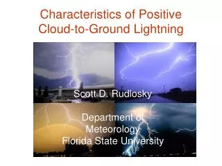
Motivation • Short term 0-1hr warning for intense cloud-to-ground lightning is valuable to the National Weather Service • Real-time ground truth available • Real-time learning algorithm that adapts to the changing nature of storms, the near-storm environment, the season, geography, etc? lakshman@ou.edu
Observations Computed Functions Advection General Idea Target Inputs Inputs Forecast+30 Target-30 Forecast t0-30 min t0+30 min t0 lakshman@ou.edu
Inputs • Inputs are gridded fields • research has shown that the following fields may predict subsequent lightning activity: • Reflectivity at certain constant height and temperature levels • Presence of mixed phase precipitation (graupel) just above melting level • Earlier lightning activity associated with storm • To minimize radar geometry problems, all the inputs are created using 3D multiple-radar grids. Inputs Target-30 t0-30 min lakshman@ou.edu
Reflectivity at Constant T Levels • Combine data from multiple radars into a 3D multi-radar merged product • Integrate this 3D radar grid with thermodynamic data from the RUC model analysis grids • dBZ at a constant height of T=-10C is shown 3D radar grid from KMLB, KAMX, KTBW, at 1626 UTC 16 July 2004 lakshman@ou.edu
Echo top input • Maximum height of 30dBZ echo is shown 3D radar grid from KMLB, KAMX, KTBW, at 1626 UTC 16 July 2004 lakshman@ou.edu
Target • Target is a lightning density field • Computed from lightning activity in the previous 15 minutes • Advected backward by the prediction interval to account for storm movement. • So that we can do pixel-by-pixel prediction Inputs Target-30 t0-30 min lakshman@ou.edu
Target Lightning Density Field • Cloud-to-Ground (CG) lightning strikes are instantaneous • Average in space (3km, Gaussian) and time (15 min) lakshman@ou.edu
Advecting Target Backwards • We want to predict for each grid pixel • However, storms move • So, need to correct for storm movement • Storm movement estimated using K-means clustering and Kalman filtering lakshman@ou.edu
Mapping Function • We want a mapping function • Pixel-by-pixel predictor of the vector of inputs to the desired target lightning density • Must be fast enough to compute, and learn, in real-time Inputs Target-30 t0-30 min lakshman@ou.edu
Linear Radial Basis Functions • Weighted average of multi-dimensional Gaussian functions, so it is a non-linear system • If you keep xn fixed, this is a linear system. • Solve for sigma and weights by inverting a matrix lakshman@ou.edu
Mapping Function • For example, one of the inputs is dBZ at a constant height of T = -10C • This is the relationship between the reflectivity values and CG lightning activity 30 minutes later (t0 + 30 min) lakshman@ou.edu
Prediction • When predicting, gather the inputs at the current time, then use the same mapping function to make forward prediction • Then advect that forecast field forward by 30 minutes Inputs Forecast+30 Forecast t0+30 min lakshman@ou.edu
Example CG ltg Density at t0 dBZ at a constant ht of T=-10C at t0 Forecast CG ltg Density at t0 + 30 min Observed CG ltg Density at t0 + 30 min lakshman@ou.edu
Future • Test using a variety of input fields, lightning density functions, and forecast intervals • Results to be reported at a future AMS conference • If successful, may be implemented in AWIPS to serve as guidance for future NWS lightning warning products lakshman@ou.edu
Summary • Very much a work in progress • Thanks for listening! • Questions? lakshman@ou.edu