Download
1 / 1
10 likes | 161 Vues
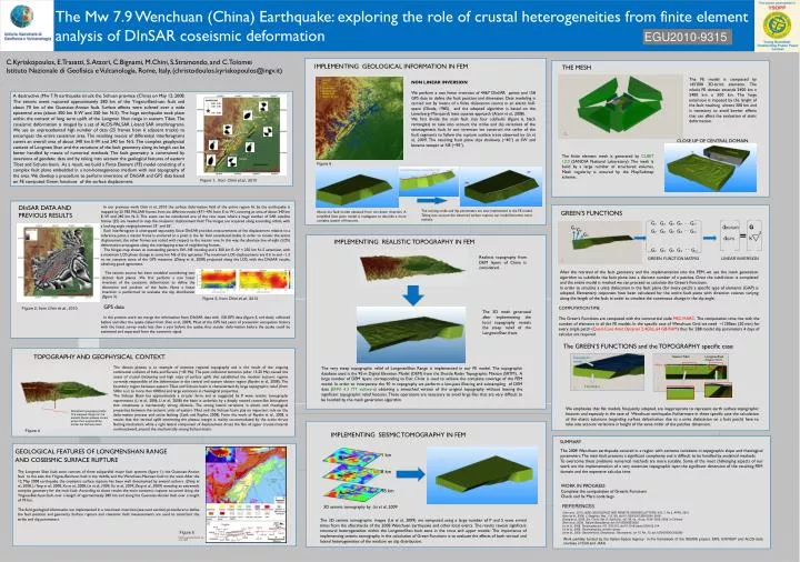
The Mw 7.9 Wenchuan (China) Earthquake: exploring the role of crustal heterogeneities from finite element analysis of DInSAR coseismic deformation. NE. SW. EGU2010-9315. C.Kyriakopoulos, E.Trasatti, S. Atzori, C.Bignami, M.Chini, S.Stramondo, and C.Tolomei

E N D
The Mw 7.9 Wenchuan (China) Earthquake: exploring the role of crustal heterogeneities from finite element analysis of DInSAR coseismic deformation NE SW EGU2010-9315 C.Kyriakopoulos, E.Trasatti, S. Atzori, C.Bignami, M.Chini, S.Stramondo, and C.Tolomei Istituto Nazionale di Geofisica e Vulcanologia, Rome, Italy, (christodoulos.kyriakopoulos@ingv.it) IMPLEMENTING GEOLOGICAL INFORMATION IN FEM THE MESH The FE model is composed by 145’000 3D-brick elements. The whole FE domain extends 2400 km x 2400 km x 500 km. The large extension is imposed by the lenght of the fault reaching almost 300 km and is necessary to avoid border effects that can affect the evaluation of static deformation. DInSAR NON LINEAR INVERSION We perform a non linear inversion of 4467 DInSAR points and 158 GPS data to define the fault position and dimension. Data modeling is carried out by means of a finite dislocation source in an elastic half-space (Okada, 1985), and the adopted algorithm is based on the Levenberg–Marquardt least squares approach (Atzori et al., 2008). We first divide the main fault into four subfaults (figure 6, black rectangles) to take into account the strike and dip variations of the seismogenetic fault. In our inversion we constrain the strike of the fault segments to follow the rupture surface trace observed by Lin et al., 2009. The resulting fault plane dips shallowly (~40°) at SW and became steeper at NE (~90°). GPS 1 Yigxiou fault 2 Beichuan fault 3 Nanba fault 4 Qingchuan fault A destructive (Mw 7.9) earthquake struck the Sichuan province (China) on May 12, 2008. The seismic event ruptured approximately 280 km of the Yingxiu-Beichuan fault and about 70 km of the Guanxian-Anxian fault. Surface effects were sufered over a wide epicentral area (about 300 km E-W and 250 km N-S). The huge earthquake took place within the context of long term uplift of the Longmen Shan range in eastern Tibet. The coseismic deformation is imaged by a set of ALOS-PALSAR L-band SAR interferograms. We use an unprecedented high number of data (25 frames from 6 adjacent tracks) to encompass the entire coseismic area. The resulting mosaic of differential interferograms covers an overall area of about 340 km E-W and 240 km N-S. The complex geophysical context of Longmen Shan and the variations of the fault geometry along its length can be better handled by means of numerical methods. The fault geometry is constrained by inversions of geodetic data and by taking into account the geological features of eastern Tibet and Sichuan basin. As a result, we build a Finite Element (FE) model consisting of a complex fault plane embedded in a non-homogeneous medium with real topography of the area. We develop a procedure to perform inversions of DInSAR and GPS data based on FE computed Green functions of the surface displacement. 4 Qingchuan 3 2 1 Beichuan Maoxian CLOSE UP OF CENTRAL DOMAIN Anxian Wenchuan Yingxiu The finite element mesh is generated by CUBIT 12.0 (SANDIA National Laboratory). The mesh is build by a large number of structured volumes. Mesh regularity is ensured by the Map/Submap scheme. Guanxian Chengdu Figure 6 Figure 5 Figure 1, from Chini et al., 2010 DInSAR DATA AND PREVIOUS RESULTS In our previous work Chini et al., 2010 the surface deformation field of the entire region hit by the earthquake is mapped by 25 FBS PALSAR frames from six different tracks (471–476 from E to W), covering an area of about 340 km E–W and 240 km N–S. This event can be considered one of the rare cases where a huge number of SAR satellite frames (25) are needed to map the coseismic displacement field. The images are acquired along ascending orbits, with a looking angle ranging between 33° and 36°. Each interferogram is unwrapped separately. Since DInSAR provides measurements of the displacement relative to a reference point, a master frame is anchored to a point in the far field considered stable. In order to mosaic the entire displacement, the other frames are scaled with respect to the master one. In this way, the absolute line-of-sight (LOS) deformation propagates along the overlapping areas of neighboring frames. The fringes map shows an outstanding pattern SW–NE trending and a 300 km E–W × 250 km N–S extension, with a maximum LOS phase change at some km NE of the epicenter. The maximum LOS displacements are 0.6 m and −1.3 m; we compare some of the GPS measures (Zhang et al., 2008) projected along the LOS, with the DInSAR results, obtaining good agreement. GPS data In the present work we merge the information from DInSAR data with 158 GPS data (figure 5, red dots), collected before and after the quake (taken from Shen et al., 2009). Most of the GPS had years of preseismic occupation history with the latest survey made less than a year before the quake, thus secular deformation before the quake could be estimated and separated from the coseismic signal. The varying strike and dip parameters are now implmented in the FE model. Taking into account the observed surface rupture our model becomes more realistic. GREEN’S FUNCTIONS Above the fault model obtained from non-linear inversion. A simplified fault plane model is inadeguate to describe a more complex system of fractures. G11 G12 G13 G14 … G1m dDInSAR G G11 G21 … G21 G22 G23 G24 G2m 2 G31 dGPS k IMPLEMENTING REALISTIC TOPOGRAPHY IN FEM … Gn1 Gn2 Gn3 Gn4 Gnm Realistic topography from DEM layers of China is considered. GREEN FUNCTION MATRIX LINEAR INVERSION After the retrieval of the fault geometry and the implementation into the FEM, we use the mesh generation algorithm to subdivide the fault plane into a discrete number of n patches. Once the subdivision is completed and the entire model is meshed we can proceed to calculate the Green’s Functions. In order to simulate a unite dislocation in the fault plane (for every patch) a specific type of elements (GAP) is adopted. Elementary responses have been calculated for the entire fault plane with direction cosines variyng along the length of the fault in order to simulate the continuous change in the dip angle. The seismic source has been modeled considering two distinct fault planes .We first perform a non linear inversion of the coseismic deformation to define the dimension and position of the faults. Next a linear inversion is performed to evaluate the slip distribution (figure 3). Figure 3, from Chini et al., 2010 COMPUTATION TIME The Green’s Functions are computed with the commercial code MSC.MARC. The computation time rise with the number of elements in all the FE models. In the specific case of Wenchuan Grid we need ~1200sec (20 min) for every single patch (Quad-Core Amd Opteron 2.4Ghz, 64 GB RAM) thus for 288 model slip parameters 4 days of calculus are required. Figure 2, from Chini et al., 2010 The 3D mesh generated after implementing the local topography reveals the steep relief of the LongmenShan front. The GREEN’S FUNCTIONS and the TOPOGRAPHY specific case TOPOGRAPHY AND GEOPHYSICAL CONTEXT Eastern Tibet LomgmenShan (Pengguan Massif) Topographic model ~4500 m The tibetan plateau is an example of extreme regional topography and is the result of the ongoing continental collision of India and Eurasia (~45 Ma). The post collisional tectonics (after 15-20 Ma) caused the onset of crustal thickening and high rates of surface uplift that established the modern tectonic regime currently responsible of the deformation in the central and eastern tibetan region (Royden et al., 2008). The boundary region between eastern Tibet and Sichuan basin is characterized by large topographic relief (from 500m a.s.l. to more than 4000m) and large variations in rheological properties. The Sichuan Basin has approximately a circular form, and as suggested by P wave seismic tomography experiments (Li et al., 2006, Li et al., 2008) the basin is underlain by a deeply rooted craton-like lithosphere that constitutes a mechanically strong obstacle. The strong lateral variations in elastic and rheological properties between the tectonic units of eastern Tibet and the Sichuan basin play an important role on the deformation process and active faulting (Cook and Royden, 2008). From the work of Royden et al., 2008, it results that the vertical uplift interesting the plateau margin is mainly accommodated by the active thrust faulting mechanism, while a right lateral component of displacement drives the flux of upper crustal material northeastward, around the mechanically strong Sichuan basin. The very steep topographic relief of LongmenShan Range is implemented in our FE model. The topographic database used is the 90 m Digital Elevation Model (DEM) from the Shuttle Radar Topographic Mission (SRTM). A large number of DEM layers corresponding to East China is used to achieve the complete coverage of the FEM model. In order to incorporate the 90 m topography we perform a low-pass filtering and subsampling of DEM data (ENVI 4.3 ITT software) obtaining a smoothed version of the original topography without loosing the significant topographic relief features. These operations are necessary to avoid large files that are very difficult to be handled by the mesh generation algorithm. Flat Model EASTERN TIBET SICHUAN BASIN We emphasize that flat models, frequently adopted, are inappropriate to represent earth surface topographic features and especialy in the case of Wenchuan earthquake. Futhermore in these specific case the calculation of the elastic solutions (regarding surface deformation due to a unite dislocation on a fault patch) have to take into account variations in height of the same order of the patches dimension. Simplified topography profile The steepest margin on the eastern tibetan plateau occurs where the LongmenShan border the Sichuan basin Figure 4 IMPLEMENTING SEISMIC TOMOGRAPHY IN FEM SUMMARY GEOLOGICAL FEATURES OF LONGMENSHAN RANGE AND COSEISMIC SURFACE RUPTURE The 2008 Wenchuan earthquake occured in a region with extreme variations in topographic slope and rheological parameters. The main fault presents a significant complexity and is difficult to be handled by analytical methods. To overcome these problems numerical methods are more suitable. Some of the most challenging aspects of our work are the implementation of a very extensive topographic layer, the significant dimension of the resulting FEM domain and the expensive calculus time. 1 km 8 km The Longmen Shan fault zone consists of three subparallel major fault systems (figure 1): the Guanxian-Anxian fault to the east, the Yingxiu-Beichuan fault in the middle, and the Wenchuan-Maowen fault to the west. After the 12, May 2008 earthquake the coseismic surface rupture has been well documented by several authors (Deng et al., 2008, Li Yong et al., 2008, Xu et al., 2008, Lin et al., 2009, Xu et al., 2009, Zeng et al., 2009) revealing an extremely complex geometry for the main fault. According to these results the main coseismic rupture occurred along the Yingxiu-Beichuan fault, over a length of approximately 280 km and along the Guanxian-Anxian fault over a length of 70 km. The field geological information are implemented in a non-linear inversion (see next section) procedure to define the fault position and geometry. Surface rupture and coseismic field measurements are used to constraint the strike and dip parameters. WORK IN PROGRESS Complete the computation of Green’s Functions Check and fix Marc code bugs 18 km REFERENCES 3D seismic tomography by Lei et al., 2009 Chini et al., 2010, IEEE GEOSCIENCE AND REMOTE SENSING LETTERS, VOL 7, No 2, APRIL 2010 Atzori et al., 2008, J. Geophys. Res., 113, B9, doi:10.1029/2007JB005504, 2008 Zhang et al., 2008, Sci. China, Set. D, Earth Sci., vol. 38, no. 10, pp. 1195–1206, 2008. in Chinese Shen et al., 2009, Nature Geoscience, doi:10.1038/NGEO636 Lin et al., 2009, Tectonophysics, 471, 203-215, doi:10.1016/j.tecto.2009.02.014 Lin et al., 2009, Tectonophysics, article in press Lei et al., 2009, Geochemistry, Geophysics, Geosystems, vol 10, No, 10, doi:1029/2009GC002590 The 3D seismic tomographic images (Lei et al., 2009)are computed using a large number of P and S wave arrival times from the aftershocks of the 2008 Wenchuan earthquake and other local events. The results reveals significant structural heterogeneities within the LongmenShan fault zone in the crust and upper mantle. The importance of implementing seismic tomography in the calculation of Green Functions is to evaluate the effects of both vertical and lateral heterogeneities of the medium on slip distribution. Figure 5 Surface rupture desribed by Lin et al., 2009 Work partially funded by the Italian Space Agency in the framework of the SIGRIS project. ERS, ENVISAT and ALOS data courtesy of ESA and JAXA.