Download
1 / 12
120 likes | 128 Vues
First-Time User Guide Drift-Diffusion Lab v1.31. Saumitra Raj Mehrotra*, Ben Haley, Gerhard Klimeck Network for Computational Nanotechnology (NCN) Electrical and Computer Engineering http://nanohub.org/resources/ semi *smehrotr@purdue.edu. Table of Contents.

E N D
First-Time User Guide Drift-Diffusion Lab v1.31 Saumitra Raj Mehrotra*, Ben Haley, Gerhard Klimeck Network for Computational Nanotechnology (NCN) Electrical and Computer Engineering http://nanohub.org/resources/semi *smehrotr@purdue.edu
Table of Contents • Introduction 3 • What is drift and diffusion? • What can be done with the Drift-Diffusion lab? • Drift-Diffusion Lab: input parameters 5 • Simulation Runs 6 • Example 1: A walk-through of a “drift” problem • Example 2: A walk-through of a “diffusion” problem • Final Comments on the Operation of the Tool 11 • Reference 12
Introduction: What is Drift and Diffusion ? Diffusion – movement of carriers from a region of a higher concentration to a region of a lower concentration Drift –under movement of carriers application of electric field [1] [1] J(x) : Current Density (A/cm-2) q : Charge of an Electron (C) D : Diffusion Constant (cm2/s) n : Carrier Density (cm-3) J(x) : Current Density (A/cm-2) q : Charge of an Electron (C) µ : Carrier Mobility (cm2/V.s) E : Electric Field (V/cm)
Introduction: What can be Done with the Drift-Diffusion Lab? Simulate multiple experiments with a combination of Drift and Diffusion mechanisms. simulate drift with applied bias simulate diffusion by shining light Light Shine Semiconductor Slab Applied Bias
Input Parameters for the Tool • Choose Experiment: • Apply bias only • define bias value • Shine light at edge • define generation rate (/cm3.s) • define depth of penetration • Shine light at top • define the region at top for light shine • Shine light at edge and apply bias • Shine light at top and apply bias • Simulation Setup: • Material (Si/Ge/GaAs) • Minority carrier lifetime (us) • Length of slab (um) • Type of doping (n/p type) • Doping level (/cm3) • Turn ON/OFF surface recombination • Set operation temperature (K) Light Shine Applied Bias
Example 1: A Walk-through of a ‘Drift’ Problem • This tool can be used to estimate low field electron mobilities μn for bulk Si, Ge and GaAs. Consider the following example: Assume a 1 m long semiconductor N type doped at 1e15/cm3 Choose the Experiment: 1. Apply bias only
A Walk-through of a ‘Drift’ Problem, cont’d Choose material – Si/Ge/GaAs Let the experiment be at room temperature – 300K and the bias ranges from 0-0.6V. E=6000 V/cm “0.6V applied across 1m” Set surface recombination velocity to a high value to obtain an ideal contact.
A Walk-through of a ‘Drift’ Problem, cont’d Velocity saturation leads to the current being saturated at a high electric field GaAs Calculated electron mobilities at 300K for Nd=1e15/cm3 doping level: Si –1281 cm-2 / V.s Ge - 3100 cm-2 / V.s GaAs - 5093 cm-2 / V.s Ge Si J=q.n.μ.E slope gives us μ Energy band at equilibrium and at high bias
Example 2: A Walk-through of a ‘Diffusion’ Problem • This tool can be used to calculate the coefficient of diffusion for electrons Dn in Silicon. • You would perform the experiment on a P type doped at 1e14/cm3, 5 µm long Si bar. • Set minority carrier lifetimes as τ =10 ps for electrons and holes. • Set generation rate, G = 2e20 /cm3s and shine between 2.4~2.6 um. • Set ON recombination velocity on both contacts. We can now simulate the way excess electrons, generated at the left edge, would diffuse to the right!
A Walk-through of a ‘Diffusion’ Problem, cont’d Quasi fermi level for electrons shift up because of extra minority carriers! Electron and hole carriers are shown to the left. The extra electrons generated at the center diffuse on either side. Diffusion Length,L = (Dn .τ) ½ Estimated here Dn ~ 40 cm2/s [1]
Final Comments • More can be studied about drift and diffusion through using different experiments. • Semiconductor slabs longer than 10 µm would take longer to generate results, and in some cases, would lead to a convergence error. • Minority carrier lifetimes might need to be tweaked to shorten the diffusion length and so that the whole device might visualize. • A high surface recombination velocity defines an ideal contact.
Reference [1] Semiconductor Device Fundamentals by Robert F. Pierret This tool is powered by PADRE (Pisces And Device Replacement) and developed by Mark Pinto & Kent Smith at AT&T Bell Labs.