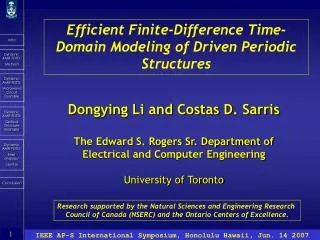
Efficient Finite-Difference Time-Domain Modeling of Driven Periodic Structures

1. Efficient Finite-Difference Time-Domain Modeling of Driven Periodic Structures Dongying Li and Costas D. Sarris The Edward S. Rogers Sr. Department of Electrical and Computer Engineering University of Toronto Research supported by the Natural Sciences and Engineering Research Council of Canada (NSERC) and the Ontario Centers of Excellence.

2. Outline • Introduction • Motivation of the research • Previous work • Theory • Floquet's theorem and sine-cosine periodic boundary condition (PBC) • Array scanning method • Numerical Examples • Printed structure on PBG substrates • Transmission-line (TL) metamaterials • Conclusions and future work

3. Motivation • Metamaterials • Simultaneous negative • Split-ring resonator (SRR), strip-wire, transmission-line (TL) grid • Design of metamaterials closely related to periodic structure modeling • periodic structures modeling

4. Marching in time scheme Finite-Difference Time-Domain (FDTD) Yee’s cell FDTD: Domain decomposition in “Yee cells”; marching in time Intro Example : FDTD discretization of

5. Example: Non-uniform mesh for microstrip Mesh Refinement in FDTD • Local mesh refinement schemes: Embedding a locally dense mesh into a coarse mesh. • Mesh refinement guided by physical intuition; statically defined at the start of the simulation. • Side-effect: stability. • Sample references: Intro I. S. Kim and W. J. R. Hoefer, MTT-T, June 1990. S. S. Zivanovic, K. S.Yee, and K. K. Mei, MTT-T, Mar. 1991. M. W. Chevalier, R. J. Luebbers, and V. P. Cable, AP-T, Mar. 1997. M. Okoniewski, E. Okoniewska, and M. A. Stuchly, AP-T, Mar. 1997.

6. Why Dynamic Mesh Refinement • Time-domain methods register the evolution of a source pulse and its retro-reflections in a given domain. • Edges, high-dielectric regions etc. are not continuously illuminated during an FDTD simulation; local mesh refinement around them is NOT always necessary. Intro Wideband source Simulated Structure Absorbing boundary

7. Previous Work • Adaptive Mesh Refinement [Berger, Oliger, J. Comput. Physics,1984]: • Computational fluid dynamic tool for hyperbolic PDEs. • Performs selective mesh refinement by factors of 2. • Allows for the dynamic re-generation of coarse/dense mesh regions. • Moving-Window FDTD (MW-FDTD, Luebbers et al., Proc. IEEE AP-S, June 2003): • Single moving window of fixed width, velocity tracking a forward wave in a wireless link. Intro

8. Dynamically AMR-FDTD: Overview • Key features of this work on Dynamically Adaptive Mesh Refinement (AMR)-FDTD • Combination of the FDTD technique with the AMR algorithm. • Implementation of a three-dimensional adaptive, moving mesh. Dynamic AMR-FDTD: Method

9. AMR-FDTD: Root/Child Meshes • The AMR-FDTD starts by covering the computational domain in a coarse mesh (called root mesh), of Yee cell dimensions • Every NAMR time steps, checks whether mesh refinement is needed at any part of the domain. Dynamic AMR-FDTD: Method

10. AMR-FDTD: Root/Child Meshes (cont-d) • Clustering together cells that have been “flagged” for refinement, it generates a child mesh that covers them, with cell sizes • Recursively, child meshes can be refined by a factor of two if flagged at a later check. Dynamic AMR-FDTD: Method

11. AMR-FDTD: Root / Child Meshes (cont-d) • Mesh generation corresponds to atree structure. Dynamic AMR-FDTD: Method A: Level 1 (Root) Mesh B1, B2,…, B5: Level 2 Meshes C1, C3: Level 3 Meshes MESH TREE Yee cells Level 1 Level 2 Level 3

12. AMR-FDTD: Time Stepping • Stability condition for the root mesh: • Courant number s < 1. • Keeping the same Courant number in all meshes, the time step of level M mesh is: • Note: Minimum cell size affects the time step of the corresponding mesh level only (asynchronous updates). Field Updates in AMR-FDTD Dynamic AMR-FDTD: Method

13. Adaptive Mesh Refinement • Each NAMR time steps, the mesh tree is regenerated. • Method: Calculate energy in each Yee cell and then gradient throughout the domain. Dynamic AMR-FDTD: Method

14. Adaptive Mesh Refinement (cont-d) • If both of the following conditions are met : Dynamic AMR-FDTD: Method : predefined thresholds cell (i, j, k) of the root mesh is flagged for refinement • First criterion: Captures energy gradient peaks. • Second criterion: Prevents numerical noise (at later stages) from triggering spurious refinements.

15. Adaptive Mesh Refinement: Clustering • Mesh Refinement is extended at a distance D around a flagged cell: • This accounts for wave propagation within the mesh refinement time window of NAMR time steps. • Flagged cells are clustered in rectangular regions following the algorithm of [Berger and Rigoutsos, IEEE Trans. Systems, Man, Cybernetics, Sept. 1991]. : “spreading” factor Dynamic AMR-FDTD: Method Flagged cells

16. Application: Microstrip Low-Pass Filter* Vertical electric field magnitude Dynamic AMR-FDTD: Microwave Circuit Example A=40mm, B1=2mm, B2=21mm, W=3mm, 0.8mm substrate of er=2.2 *From Sheen et al, IEEE MTT-T, July 1990. Time = 0 Number of Child Meshes = 1 Refined volume/total volume = 0.043

17. Application: Microstrip Low-Pass Filter Intro Vertical electric field magnitude Dynamic AMR-FDTD: Method Dynamic AMR-FDTD: Microwave Circuit Example A=40mm, B1=2mm, B2=21mm, W=3mm, 0.8mm substrate of er=2.2 Dynamic AMR-FDTD: Error analysis/ control Conclusion Time = 100Dt Number of Child Meshes = 1 Refined volume/total volume = 0.134

18. Application: Microstrip Low-Pass Filter Vertical electric field magnitude Dynamic AMR-FDTD: Microwave Circuit Example A=40mm, B1=2mm, B2=21mm, W=3mm, 0.8mm substrate of er=2.2 Time = 200Dt Number of Child Meshes = 1 Refined volume/total volume = 0.525

19. Application: Microstrip Low-Pass Filter Vertical electric field magnitude Dynamic AMR-FDTD: Microwave Circuit Example A=40mm, B1=2mm, B2=21mm, W=3mm, 0.8mm substrate of er=2.2 Time = 500Dt Number of Child Meshes = 3 Refined volume/total volume = 0.442

20. Application: Microstrip Low-Pass Filter Vertical electric field magnitude Dynamic AMR-FDTD: Microwave Circuit Example A=40mm, B1=2mm, B2=21mm, W=3mm, 0.8mm substrate of er=2.2 Time = 800Dt Number of Child Meshes = 3 Refined volume/total volume = 0.28

21. Evolution of Child Meshes Dynamic AMR-FDTD: Microwave Circuit Example In the long-time regime, AMR-FDTD is equivalent to a root-mesh based uniform mesh FDTD (reason for no late-time instability). Coverage=Volume of child meshes / total volume of the domain

22. Late-Time Regime Dynamic AMR-FDTD: Microwave Circuit Example No late-time instability observed !

23. Optical applications: Power Splitter • Dimensions are given in microns. • Dielectric constants: Dynamic AMR-FDTD: Optical Structure Example

24. Power Splitter: Time-Domain Results Port 2 • AMR-FDTD with four levels Dynamic AMR-FDTD: Optical Structure Example Port 3

25. Power Splitter: Numerical Results (cont-d) • Error Metric: Dynamic AMR-FDTD: Optical Structure Example

26. Power Splitter: Wave front Tracking Dynamic AMR-FDTD: Optical Structure Example

27. Dielectric Ring Resonator* (4-level AMR) Port 2 Dynamic AMR-FDTD: Optical Structure Example *Hagness et al., IEEE J. Lightwave Tech., vol. 15, pp. 2154-2165, Nov. 1997.

28. Dielectric Ring Resonator (cont-d) Dynamic AMR-FDTD: Optical Structure Example

29. Dielectric Ring Resonator: Late-time regime Dynamic AMR-FDTD: Optical Structure Example No late-time instability observed !

30. Determining the AMR Parameters • Objective: Produce clear guidelines for the determination of the controlling parameters of the AMR-FDTD. • Methodology: 2-D TE case studies run; error compared to reference simulation (densely gridded FDTD) was measured at probe points distributed throughout the computational domain, over time: • This procedure is aimed at rendering the error bound estimates independent of the simulated structure. Dynamic AMR-FDTD: Error analysis/ control

31. Choice of thresholds qe, qg Errors from several numerical experiments as a function of the thresholds qe, qg are collected. Error curves are fitted with the function: Dynamic AMR-FDTD: Error analysis/ control • Error bounds for the cases when qe=0 orqg=0 are derived • along with the constants C1-C4.

32. Effect of window of mesh refinement NAMR • Every NAMR time steps, cells that need mesh refinement are “flagged”. • Mesh Refinement is extended at a distance D around a flagged cell • to account for wave propagation within the mesh refinement time • window: : “spreading” factor • Increasing NAMR reduces errors, but also increases simulation time (because of “spreading factor”). • A value that compromises accuracy and efficiency is NAMR=10. Dynamic AMR-FDTD: Error analysis/ control

33. Effect of number of mesh refinement levels • Keeping the resolution constant, the effect of increasing AMR levels is tested (root mesh gets coarser). • Eventually, as the number of levels increases (beyond typically 4), error and simulation time increases. • Example: Corrugated waveguide simulation Dynamic AMR-FDTD: Error analysis/ control Dimensions in microns

34. Conclusions • The dynamically AMR-FDTD implements multiple, adaptively generated sub-grids in two/three-dimensional FDTD and achieves up to two-orders of magnitude computation time savings. • The mesh generation in AMR-FDTD is a self-adaptive process, based on pre-defined accuracy parameters (CAD-oriented feature). Conclusion

35. Conclusions (cont-d) • Guidelines for the choice of the AMR parameters were provided by studying their effect on time-domain error metrics. • Future Research • Refinement of mesh refinement criteria ! • Closed-domain, evanescent-wave problems • High-order finite-differences, conformal meshing Conclusion

36. References • C.D. Sarris, Adaptive Mesh Refinement for Time-Domain Electromagnetics, Morgan&Claypool. • Y. Liu, C.D. Sarris, ``Fast Time-Domain Simulation of Optical Waveguide Structures with a Multilevel Dynamically Adaptive Mesh Refinement FDTD Approach'', IEEE/OSA J. Lightwave Technology, vol. 24, no. 8, pp. 3235-3247, Aug. 2006. • Y. Liu, C.D. Sarris, ``Efficient Modeling of Microwave Integrated Circuit Geometries via a Dynamically Adaptive Mesh Refinement (AMR)-FDTD Technique'', IEEE Trans. on Microwave Theory Tech., vol. 54, no.2, Feb. 2006.

37. Questions/Remarks? Thank you ! E-mail:cds@waves.toronto.edu

38. Field Update Flowchart: General Check the number of time steps; if it is an integer multiple of NAMR, re-generate the mesh tree. 1 Field Updates in AMR-FDTD 2 Update field grid points of the root mesh Copy fields from the root mesh to the child meshes. Update level M meshes 2M-1 times. 3 Copy fields of the child meshes back to the root mesh for the time steps of the root mesh (interpolating as needed) . 4 If maximum time step has been reached, terminate. Otherwise go back to (1). 5

39. AMR-FDTD: Mesh boundary updates • Types of boundaries Field Updates in AMR-FDTD

40. AMR-FDTD: Mesh boundary updates • Types of boundaries Field Updates in AMR-FDTD Segment ea: “Physical boundary” (PB) of a child mesh to a terminating boundary (ABC, PEC etc.).

41. AMR-FDTD: Mesh boundary updates • Types of boundaries Field Updates in AMR-FDTD Segment cd: “Sibling boundary” (SB) between child meshes of the same level (same Yee cell volume).

42. AMR-FDTD: Mesh boundary updates • Types of boundaries Field Updates in AMR-FDTD Segments ab, bc, ed: “Child-Parent boundaries” (CPB’s) between child and parent meshes.

43. : Child mesh : Parent mesh Mesh boundary updates: CPBs • Child/Parent grid points: Never collocated in space or time (always interleaved). • Transfer of field values from the one mesh to the other involves spatial and temporalinterpolations. Field Updates in AMR-FDTD

44. Field Update Flowchart: Child/Parent Connection Update H-field points in the parent mesh at (n+1/2)Dt. 1 Field Updates in AMR-FDTD Update E-field points in the parent mesh at (n+1)Dt. 2 For each child mesh, update H-field points at (n+1/4)Dt. 3 For each child mesh, obtain non-boundary E-field points at (n+1/2)Dt. 4 For each child mesh, obtain boundary E-field points at (n+1/2)Dt, invoking interpolated H-field values of the parent mesh. 5

45. Field Update Flowchart: Child/Parent Connection (cont-d) Repeat 3, 4, 5 to advance each child mesh to time step (n+1)Dt. 6 Field Updates in AMR-FDTD At regions where child/parent meshes overlap, update parent grid points by interpolating child grid points. 7 • This algorithm is recursively applied for the interconnection of higher-level child/parent meshes (for example to connect level 2 to level 3 and so on).