Download
1 / 26
980 likes | 3.04k Vues
t- and F-tests. Testing hypotheses. Overview. Distribution& Probability Standardised normal distribution t-test F-Test (ANOVA). Starting Point. Central aim of statistical tests: Determining the likelihood of a value in a sample, given that the Null hypothesis is true : P(value|H 0 )

E N D
t- and F-tests Testing hypotheses
Overview • Distribution& Probability • Standardised normal distribution • t-test • F-Test (ANOVA)
Starting Point • Central aim of statistical tests: • Determining the likelihood of a value in a sample, given that the Null hypothesis is true: P(value|H0) • H0: no statistically significant difference between sample & population (or between samples) • H1: statistically significant difference between sample & population (or between samples) • Significance level: P(value|H0) < 0.05
a/2 Distribution & Probability If we know s.th. about the distribution of events, we know s.th. about the probability of these events
Standardised normal distribution • the z-score represents a value on the x-axis for which we know the p-value • 2-tailed: z = 1.96 is 2SD around mean = 95% ‚significant‘ • 1-tailed: z = +-1.65 is 95% from ‚plus or minus infinity‘ Population Sample
Degrees of freedom (df) • Number of scores in a sample that are free to vary • n=4 scores; mean=10 df=n-1=4-1=3 • Mean= 40/4=10 • E.g.: score1 = 10, score2 = 15, score3 = 5 score4 = 10
Kinds of t-tests Formula is slightly different for each: • Single-sample: • tests whether a sample mean is significantly different from a pre-existing value (e.g. norms) • Paired-samples: • tests the relationship between 2 linked samples, e.g. means obtained in 2 conditions by a single group of participants • Independent-samples: • tests the relationship between 2 independent populations • formula see previous slide
Independent sample t-test Number of words recalled df = (n1-1) + (n2-1) = 18 Reject H0
Bonferroni correction • To control for false positives: • E.g. four comparisons:
F-tests / Analysis of Variance (ANOVA) T-tests - inferences about 2 sample means But what if you have more than 2 conditions? e.g. placebo, drug 20mg, drug 40mg, drug 60mg Placebo vs. 20mg 20mg vs. 40mg Placebo vs 40mg 20mg vs. 60mg Placebo vs 60mg 40mg vs. 60mg Chance of making a type 1 error increases as you do more t-tests ANOVA controls this error by testing all means at once - it can compare k number of means. Drawback = loss of specificity
F-tests / Analysis of Variance (ANOVA) Different types of ANOVA depending upon experimental design (independent, repeated, multi-factorial) Assumptions • observations within each sample were independent • samples must be normally distributed • samples must have equal variances
F-tests / Analysis of Variance (ANOVA) t = obtained difference between sample means difference expected by chance (error) F = variance (differences) between sample means variance (differences) expected by chance (error) Difference between sample means is easy for 2 samples: (e.g. X1=20, X2=30, difference =10) but if X3=35 the concept of differences between sample means gets tricky
F-tests / Analysis of Variance (ANOVA) Solution is to use variance - related to SD Standard deviation = Variance E.g. Set 1 Set 2 20 28 30 30 35 31 s2=58.3 s2=2.33 These 2 variances provide a relatively accurate representation of the size of the differences
F-tests / Analysis of Variance (ANOVA) Simple ANOVA example Total variability • Between treatments variance • ---------------------------- • Measures differences due to: • Treatment effects • Chance Within treatments variance -------------------------- Measures differences due to: 1. Chance
F-tests / Analysis of Variance (ANOVA) When treatment has no effect, differences between groups/treatments are entirely due to chance. Numerator and denominator will be similar. F-ratio should have value around 1.00 When the treatment does have an effect then the between-treatment differences (numerator) should be larger than chance (denominator). F-ratio should be noticeably larger than 1.00 MSbetween F = MSwithin
F-tests / Analysis of Variance (ANOVA) Simple independent samples ANOVA example F(3, 8) = 9.00, p<0.05 There is a difference somewhere - have to use post-hoc tests (essentially t-tests corrected for multiple comparisons) to examine further Placebo Drug A Drug B Drug C Mean 1.0 1.0 4.0 6.0 SD 1.73 1.0 1.0 1.73 n 3 3 3 3
F-tests / Analysis of Variance (ANOVA) Gets more complicated than that though… Bit of notation first: An independent variable is called a factor e.g. if we compare doses of a drug, then dose is our factor Different values of our independent variable are our levels e.g. 20mg, 40mg, 60mg are the 3 levels of our factor
F-tests / Analysis of Variance (ANOVA) • Can test more complicated hypotheses - example 2 factor ANOVA (data modelled on Schachter, 1968) • Factors: • Weight - normal vs obese participants • Full stomach vs empty stomach • Participants have to rate 5 types of crackers, dependent variable is how many they eat • This expt is a 2x2 factorial design - 2 factors x 2 levels
F-tests / Analysis of Variance (ANOVA) Mean number of crackers eaten Empty Full Result: No main effect for factor A (normal/obese) No main effect for factor B (empty/full) Normal 22 15 = 37 = 35 Obese 17 18 = 39 = 33
F-tests / Analysis of Variance (ANOVA) Mean number of crackers eaten Empty Full 23 22 21 20 19 18 17 16 15 14 Normal 22 15 obese Obese 17 18 normal Empty Full Stomach Stomach
F-tests / Analysis of Variance (ANOVA) Application to imaging…
F-tests / Analysis of Variance (ANOVA) Application to imaging… Early days => subtraction methodology => T-tests corrected for multiple comparisons = e.g. Pain Visual task Statistical parametric map Appropriate rest condition - =
F-tests / Analysis of Variance (ANOVA) This is still a fairly simple analysis. It shows the main effect of pain (collapsing across the pain source) and the individual conditions. More complex analyses can look at interactions between factors Derbyshire, Whalley, Stenger, Oakley, 2004
References Gravetter & Wallnau - Statistics for the behavioural sciences Last years presentation, thank you to: Louise Whiteley & Elisabeth Rounis http://www.fil.ion.ucl.ac.uk/spm/doc/mfd-2004.html Google