Download
1 / 24
240 likes | 446 Vues
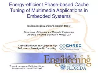
Dynamic Phase-based Tuning for Embedded Systems Using Phase Distance Mapping. Tosiron Adegbija 1 , Ann Gordon-Ross 1+ , and Arslan Munir 2 1 Department of Electrical and Computer Engineering University of Florida, Gainesville, Florida, USA

E N D
Dynamic Phase-based Tuning for Embedded Systems Using Phase Distance Mapping Tosiron Adegbija1, Ann Gordon-Ross1+,and Arslan Munir2 1Department of Electrical and Computer Engineering University of Florida, Gainesville, Florida, USA 2Department of Electrical and Computer Engineering Rice University, Houston, Texas, USA + Also Affiliated with NSF Center for High-Performance Reconfigurable Computing This work was supported by National Science Foundation (NSF) grant CNS-0953447
Introduction and Motivation • Embedded systems are pervasive, and have stringent design constraints • Constraints: Energy, size, real time, cost, etc • System optimization is challenging due to numerous tunable parameters • Tunable parameters are parameters that can be changed • E.g., cache size, associativity, line size, clock frequency, etc • Many combinations large design space • Multicore systems result in exponential increase in design space • Tradeoff competing design constraints • Design constraints: e.g., energy/performance • Resulting in Pareto optimal systems Energy How do we determine the appropriate parameter values? Pareto Optimal systems Execution time
Parameter Tuning • Parameter tuning determines appropriate parameter values • Appropriate parameter values meet optimization goals • I.e., satisfy design constraints (e.g., lowest energy, best performance) • Different applications have different parameter value requirements • Inappropriate values can waste an average of 62% in energy1 • Parameter tuningspecializes tunable parameters to the changing needs of applications • Configuration: combination of parameter values that the system is set to • Best configuration: configuration that best meets optimization goals • Much prior work in parameter tuning • However, increasingly complex systems are exponentially more challenging to tune • Our contribution: • Optimized, simplified, accurate parameter tuning for complex systems 1A. Gordon-Ross, F. Vahid, N. Dutt. Fast configurable-cache tuning with a unified second level cache. International Symposium on Low Power Electronics and Design, 2005.
2KB 2KB 2KB 2KB Way shutdown Way concatenation 2KB 2KB 2KB 2KB Configurable Line size 2KB 2KB 2KB 2KB 8 KB, 2-way 4 KB, 2-way 2KB 2KB 2KB 2KB 8 KB, 4-way base cache 2KB 2KB 2KB 2KB 16 byte physical line size 8 KB, direct-mapped 2 KB, direct-mapped Target Tuning Domain - Cache Tuning • Caches are a good candidate for optimization • Large contribution to system power, energy, performance, and area • Requirements: tunable hardware and tuninghardware A Highly Configurable Cache (Zhang ‘03) Tunable Asociativity Tunable Line Size Tunable Size
Executing in base configuration Download application Energy Cache Tuning Tunable cache TC Tuning hardware TC TC TC TC TC TC TC TC TC TC Dynamic Tuning • Determine parameter values during runtime • Online design space exploration • Tuning hardware changes tunable cache (TC) and evaluates each configuration • Tuning hardware selects best configuration (e.g., lowest energy) Cache energy savings of 62% on average! (Gordon-Ross ‘05) Lowest energy Execution time Microprocessor
Dynamic Tuning • Advantages • Adapts to the runtime operating environment • Specializes configurations to executing applications • No lengthy simulation time or complex simulation environments • Disadvantages/Challenges • Large design spaces • Must limit system intrusion/induced overheads • Power/energy/performance incurred during tuning • Accurate selection of best configuration • How are configurations evaluated? • How long must the system execute in each configuration? • Accurate detection of when a new configuration is required • I.e., a new phase of execution is entered, requiring new parameter values
Base energy Energy Consumption Application-tuned Phase-tuned Change configuration Time Phase-based Tuning • Applications have dynamic requirements during execution • Periods/intervals with similar requirements are grouped as a phase • During a phase, characteristics (e.g., cache misses, branch mispredictions, etc) remain relatively stable • Parameter tuning should coincide with phase changes • Prior work2 showed importance of this coordination–results quicklydegrade Time varying behavior for IPC, level one data cache hits, branch predictor hits, and power consumption for SPEC2000 gcc (using the integrate input set) 2A. Gordon-Ross and F. Vahid, “A self-tuning configurable cache,” IEEE Design Automation Conference, July, 2007.
PhaseClassification Variable length intervals Fixed length intervals Application x • Evaluate and group similar intervals into the same phase Profiler Conf1 Conf2 Conf4 Conf5 Conf3 So, how do we determine the best configuration for the different phases?
Energy Energy Execution time Execution time Previous Design Space Exploration Methods Exhaustive method Analytical method Heuristic method Tuning overhead Energy Energy Energy Energy Execution time Possible Cache Configurations Possible Cache Configurations Possible Cache Configurations Tuning overhead Computationally complex/not dynamic
Contributions • We introduce phase distance mapping (PDM) • Low overhead, dynamic method for determining a phase’s best configuration • No design space exploration! • Phase Characterization determines a phase’s best configuration • Best configuration determination: • Known phase: best configuration and characteristics are recorded • New phase: measure characteristics dynamically • Phase distance: difference between known and new phases’ characteristics • Distance predicts/determine the new phase’s best configuration • PDM orchestrated by phase characterization hardware: • Tuner • Phase classification module • Phase distance mapping module • Phase history table
Phase Tuning Architecture for a Sample Dual-Core System Processor core 1 Instruction Cache Instruction Cache L1 L1 Changes the tunable hardware and evaluates each configuration Data Cache Data Cache On-chip components Phase characterization hardware Tuner Main Memory Phase classification module Phase history table Phase distance mapping module Lookup table Groups similar intervals into phases Processor core 2 Stores phase characteristics and configurations Determines a new phase’s best configuration
Phase Characterization Used for comparison. Best configuration determined a priori or at runtime. • PDM is part of phase characterization • Determines the best configuration for a Phase, Pi Base phase, Pb Pb Phase classification Phases/ phase characteristics Phase history table Phase P1 executed Pb P1 CPb CPb x CP1 x CP1 P2 P1 P1 New phase, P1 x P3 P2 P4 P3 x x P4 Phase Distance Mapping CP1 P1configuration, CP1
Phase Distance Mapping (PDM) New phase Base phase Phase Pi Ci ?? d (Pb, Pi) Phase distance Configuration Estimation
Configuration Estimation • Configuration estimation is the most important part of PDM • Developed empirically • Uses the phase distance d (Pb,Pi) toestimate the configuration of Phase, Pi, based on the configuration of the base phase, Pb • Threshold values • Point of diminishing returns: parameter value at which further increases in the value may result in increased energy consumption or reduced performance • Size, associativity and line size threshold values: • CTHR, ATHR, LTHR • Distance windows • Characteristic ranges that represent a phase’s configuration distance from the base phase • Pi’s configuration distance from Pb when changing a parameter’s value
Configuration Estimation • Distance windows • Each window has an upper and lower bound, and every phase distance, d (Pb,Pi) is bounded by at least one distance window • Relate directly to the characteristics used to evaluate d (Pb,Pi), e.g., cache miss rates • For our experiments, we have 7 distance windows • Base phase: image rotation application • R1 = [0,0.25], R2 = (0.25,0.5], R3 = (0.5,0.75], R4 = (0.75,1.25], R5 = (1.25,1.5], R6 = (1.5,2.5], R7 = (2.5,∞] • Configuration estimation algorithm • Inputs: CB, AB, LB, CMIN, CMAX, AMIN, AMAX, LMIN, LMAX, CTHR, ATHR, LTHR, R1, R2, R3, R4, R5, R6, R7; Outputs: CI, AI, LI • First initialize default values • CI = CB, AI = AB, LI = LB • Determine which distance window d (Pb,Pi) maps to, and determine Pi’s best configuration based on the configuration distance for the corresponding distance window
Configuration Estimation Inputs stored in the lookup table Cb= 4KB; Ab= 4; Lb= 64; CMAX = 8KB; CMIN = 2KB, AMAX = 4; AMIN = 2; LMAX = 64B; LMIN = 16B; CTHR = 8KB; ATHR = 2; LTHR = 64B; R1 – R7 Phase Pi Base phase Pb Pb Pi Initialize default values Ci= 8KB Ai = 4 Li = 32 Ci= 4KB Ai = 4 Li = 64 Ci= ?? Ai = ?? Li = ?? Cb= 4KB Ab = 4 Lb = 64 Pi’s configurations Phase distance d (Pb, Pi) = 1.08 R4 R2 R3 R1
Experimental Setup • Design space • Level 1 instruction and data caches: cache sizes (2kB 8kB); line sizes (16B64B); associativities(direct-mapped4-way) • Base cache configuration: • Level 1 Instruction and data caches: cache size (8kB); line size (64B); associativity (4-way) • Simulations • Used GEM5 to gather cache miss rates • Used McPAT to calculate power consumption • Energy Delay Product (EDP) as evaluation metric = system_power * phase_running_time2 = system_power * (total_phase_cycles/system_frequency)2 • 16 workloads from EEMBC Multibench Suite • Image processing, MD5 checksum, networking, Huffman decoding • Each workload represented a phase
Experimental Setup • Optimal configurations determined by exhaustive search • Used for comparison with PDM results • Drove simulations and algorithm using Perl scripts
Results 47% • Using Phase 1 as the base phase • EDP savings calculated with respect to the base configuration • PDM achieved 26% average EDP savings overall • Savings as high as 47% for Phase 5 • On average, within 3% of the optimal 26% Base phase Does the choice of the base phase affect the results?
Results • Using Phase 7 as the base phase • EDP savings calculated with respect to the base configuration • PDM achieved average EDP savings of 22% • Highest savings reduced to 38% • On average, within 7% of the optimal 38% 22% Base phase Best results if base phase is from application domain that makes up majority of applications executed on the system
Conclusions • We introduced phase distance mapping (PDM) • Low overhead and dynamic method for phase-based tuning • Directly determines a phase’s best configuration • No design space exploration! • Average EDP savings of 26% • Future work • Quantify and evaluate the area, energy, and performance overheads of PDM • Apply phase distance mapping to more complex systems • E.g., heterogeneous cores with more tunable parameters • Increase adaptability of configuration estimation algorithm • More reactive to runtime application execution requirements • More general for a wider variety of application domains