Download
1 / 15

E N D
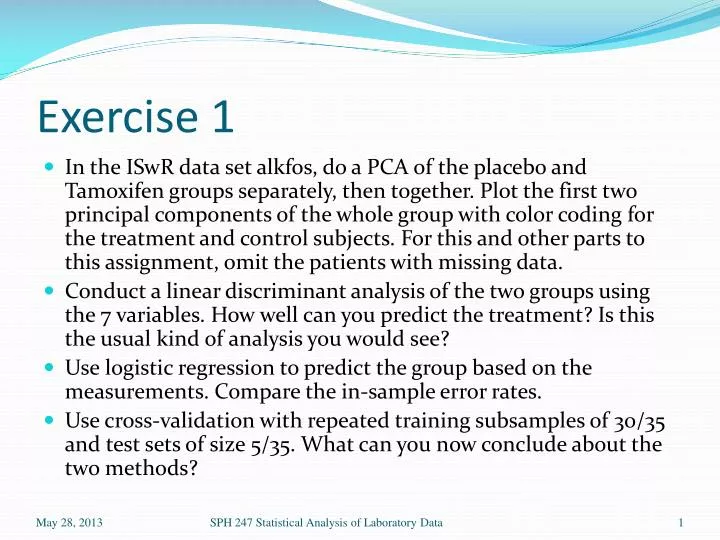
Exercise 1 • In the ISwR data set alkfos, do a PCA of the placebo and Tamoxifen groups separately, then together. Plot the first two principal components of the whole group with color coding for the treatment and control subjects. For this and other parts to this assignment, omit the patients with missing data. • Conduct a linear discriminant analysis of the two groups using the 7 variables. How well can you predict the treatment? Is this the usual kind of analysis you would see? • Use logistic regression to predict the group based on the measurements. Compare the in-sample error rates. • Use cross-validation with repeated training subsamples of 30/35 and test sets of size 5/35. What can you now conclude about the two methods? SPH 247 Statistical Analysis of Laboratory Data
Exercise 2 • In the ISwR data set alkfos, cluster the data based on the 7 measurements using hclust(), kmeans(), and Mclust(). • Compare the 2-group clustering with the placebo/Tamoxifen classification. SPH 247 Statistical Analysis of Laboratory Data
> alkfos2 <- na.omit(alkfos) # omits missing values > pc1 <- prcomp(alkfos2[alkfos2[,1]==1,2:8],scale=T) > pc2 <- prcomp(alkfos2[alkfos2[,1]==2,2:8],scale=T) > pc.all <- prcomp(alkfos2[,2:8],scale=T) Standard deviations: [1] 2.3731316 0.7123154 0.6122286 0.4955545 0.3208553 0.2954631 0.2240720 Rotation: PC1 PC2 PC3 PC4 PC5 PC6 PC7 c0 0.3484871 -0.54632917 0.6016554 0.21896409 0.39427330 -0.106360261 0.05816212 c3 0.3887022 0.16108868 0.4384481 0.06722018 -0.75501296 0.184741080 -0.14843167 c6 0.3418856 0.76808477 0.2118390 -0.03486734 0.48709933 0.097438042 -0.01756660 c9 0.4064443 -0.02858575 -0.1832107 -0.27713072 -0.12380851 -0.132875647 0.83104381 c12 0.3809874 -0.22109261 -0.1586836 -0.74610277 0.08094328 -0.004681993 -0.46641516 c18 0.3913700 0.07215108 -0.3589670 0.40921911 -0.07419710 -0.689796022 -0.25294738 c24 0.3834877 -0.17525921 -0.4618380 0.38129961 0.09926056 0.671987832 -0.04601444 > plot(pc.all) > plot(pc.all$x,col=alkfos2[,1]) SPH 247 Statistical Analysis of Laboratory Data
> library(MASS) > alkfos.lda <- lda(alkfos2[,2:8],grouping=alkfos2[,1]) > alkfos.lda Call: lda(alkfos2[, 2:8], grouping = alkfos2[, 1]) Prior probabilities of groups: 1 2 0.6 0.4 Group means: c0 c3 c6 c9 c12 c18 c24 1 156.7143 161.8571 173.9048 158.4286 163.8571 164.3333 163.2857 2 164.2143 125.1429 123.7143 118.7143 117.2857 130.7857 134.8571 Coefficients of linear discriminants: LD1 c0 0.0618073455 c3 -0.0329471378 c6 0.0004421163 c9 -0.0232320119 c12 -0.0248954902 c18 0.0113410946 c24 0.0003473940 SPH 247 Statistical Analysis of Laboratory Data
> plot(alkfos.lda) > alkfos.pred<- predict(alkfos.lda) > table(alkfos2$grp,alkfos.pred$class) 1 2 1 20 1 2 0 14 34 in 35 correct. SPH 247 Statistical Analysis of Laboratory Data
> alkfos.glm<- glm(as.factor(grp) ~ 1,data=alkfos2,family=binomial) > step(alkfos.glm,scope=formula(~ c0+c3+c6+c9+c12+c18+c24),steps=2) Start: AIC=49.11 as.factor(grp) ~ 1 Df Deviance AIC + c6 1 38.475 42.475 + c12 1 39.116 43.116 + c9 1 39.484 43.484 + c3 1 41.721 45.721 + c18 1 43.291 47.291 + c24 1 44.093 48.093 <none> 47.111 49.111 + c0 1 46.869 50.869 Step: AIC=42.47 as.factor(grp) ~ c6 SPH 247 Statistical Analysis of Laboratory Data
> alkfos.glm<- glm(as.factor(grp) ~ 1,data=alkfos2,family=binomial) > step(alkfos.glm,scope=formula(~ c0+c3+c6+c9+c12+c18+c24),steps=2) Step: AIC=42.47 as.factor(grp) ~ c6 Df Deviance AIC + c0 1 24.281 30.281 <none> 38.475 42.475 + c18 1 37.286 43.286 + c24 1 37.509 43.509 + c12 1 37.545 43.545 + c3 1 38.113 44.113 + c9 1 38.128 44.128 - c6 1 47.111 49.111 Step: AIC=30.28 as.factor(grp) ~ c6 + c0 We used step limited to two steps to avoid a model with undetermined coefficients. Once the predictions are perfect (with three or more variables in this case), nothing can be distinguished. SPH 247 Statistical Analysis of Laboratory Data
alkfos.lda.cv <- function(ncv,ntrials) { require(MASS) data(alkfos) alkfos2 <- na.omit(alkfos) n1 <- dim(alkfos2)[1] nwrong <- 0 npred <- 0 for (i in 1:ntrials) { test <- sample(n1,ncv) test.set <- data.frame(alkfos2[test,2:8]) train.set <- data.frame(alkfos2[-test,2:8]) lda.ap <- lda(train.set,alkfos2[-test,1]) lda.pred <- predict(lda.ap,test.set) nwrong <- nwrong + sum(lda.pred$class != alkfos2[test,1]) npred <- npred + ncv } print(paste("total number classified = ",npred,sep="")) print(paste("total number wrong = ",nwrong,sep="")) print(paste("percent wrong = ",100*nwrong/npred,"%",sep="")) } SPH 247 Statistical Analysis of Laboratory Data
alkfos.glm.cv <- function(ncv,ntrials) { require(MASS) data(alkfos) alkfos2 <- na.omit(alkfos) alkfos2$grp <- as.factor(alkfos2$grp) n1 <- dim(alkfos2)[1] nwrong <- 0 npred <- 0 for (i in 1:ntrials) { test <- sample(n1,ncv) test.set <- alkfos2[test,] train.set <- alkfos2[-test,] glm.ap <- glm(grp ~ 1,data=train.set,family=binomial) glmstep.ap <- step(glm.ap,scope=formula(~ c0+c3+c6+c9+c12+c18+c24),steps=2,trace=0) glm.pred <- predict(glmstep.ap,newdata=test.set,type="response") grp.pred <- (glm.pred > 0.5)+1 nwrong<- nwrong + sum(grp.pred != test.set$grp) npred <- npred + ncv } print(paste("total number classified = ",npred,sep="")) print(paste("total number wrong = ",nwrong,sep="")) print(paste("percent wrong = ",100*nwrong/npred,"%",sep="")) } SPH 247 Statistical Analysis of Laboratory Data
Results of Cross Validation • LDA has 1 error in 35 in sample (2.9%) • Cross-Validated seven-fold this is 720/10000 = 7.2% • Stepwise logistic regression with two variables has 3 errors in 35 in sample (8.6%) • Cross-Validated seven-fold this is 1830/10000 = 18.3% SPH 247 Statistical Analysis of Laboratory Data
> ap.hc<- hclust(dist(alkfos2[,2:8])) > plot(ap.hc) > cutree(ap.hc, 2) 1 2 3 4 5 7 8 9 10 11 12 13 14 15 16 17 19 20 21 22 23 24 25 27 28 29 1 1 2 2 1 2 2 1 1 2 2 1 2 2 2 1 1 1 1 1 1 1 1 1 1 1 30 31 33 34 35 37 38 40 42 1 1 1 1 1 1 1 2 1 > table(cutree(ap.hc, 2),alkfos2$grp) 1 2 1 12 13 2 9 1 > table(kmeans(alkfos2[,2:8],2)$cluster,alkfos2$grp) 1 2 1 11 11 2 10 3 > library(mclust) > Mclust(alkfos2[,2:8]) 'Mclust' model object: best model: ellipsoidal, equal shape (VEV) with 6 components > table(Mclust(alkfos2[,2:8])$class,alkfos2$grp) 1 2 1 4 3 2 6 0 3 4 4 4 6 0 5 1 4 6 0 3 > table(Mclust(alkfos2[,2:8],G=2)$class,alkfos2$grp) 1 2 1 15 14 2 6 0 SPH 247 Statistical Analysis of Laboratory Data