Download
1 / 10
100 likes | 242 Vues
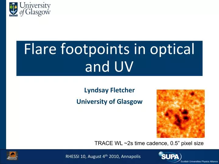
Flare footpoints in optical and UV. Lyndsay Fletcher University of Glasgow. TRACE WL ~2s time cadence, 0.5” pixel size. RHESSI 10, August 4 th 2010, Annapolis. TRACE WL, UV & RHESSI FOOTPOINTS. Yellow – WL enhancements: Green - RHESSI pixons background image – 1700A intensity.

E N D
Flare footpoints in optical and UV Lyndsay Fletcher University of Glasgow TRACE WL ~2s time cadence, 0.5” pixel size RHESSI 10, August 4th 2010, Annapolis
TRACE WL, UV & RHESSI FOOTPOINTS Yellow – WL enhancements: Green - RHESSI pixons background image – 1700A intensity RHESSI sources are a subset of WL sources (in this event – imaging problems?) WL sources are a subset of UV sources
Why don’t we see ribbons in HXRs? Why do we see small numbers of footpoints, not ribbons? Well, sometimes we do. But rarely (Liu et al 2007) Why rare? 1 – RHESSI dynamic range (~10, compared to ~103 for TRACE) 2 – it’s easy to make radiation in EUV or UV (heating, weak beams..) There are locations of preferential e- acceleration: e.g. at intersection of separatrix field lines with chromosphere (Jardin et al 2009)
WL and RHESSI sources grey = Hard X-ray Black= TRACE WL Fletcher et al 07 Brightest WL sources and RHESSI sources have good temporal and spatial correspondence at impulsive phase RHESSI and TRACE WL corrected for UV
What is TRACE WL seeing? WL 1700 A TRACE WL has a broad passband including UV lines and continuum (TRACE 1700 A is a 200 A filter in the UV continuum) Uncontaminated optical continuum flare measurements are rarer.
MDI WLF (Potts et al. 2010) MDI images are made in the continuum near 6768 A High res observations have 0.”75 px WL image Difference MDI WLF shows strong compact sources and a more diffuse, long-lasting component Analysis of photospheric structure visible through flare enhancement suggests emission is very optically thin
WL source dimensions SOT BFI– pixel size = 0.”053, spatial resolution – 0.”2-0.”3 G-band continuum is 4305 Å – CH molecular bandhead X3.4, magnetic field G-band Sharper leading edge (Diffuse ‘inner’ emission) Could be that Hinode SOT is resolving the WL sources - FWHM of bright G-band source = 500km (Isobe et al 2007) - width (including ‘diffuse’ emission) ~ 2” = 1500 km, length = 10”=7500km
Hinode G-band Hinode/RHESSI flare December 6 2006 analysed by Krucker et al G-band enhancement and RHESSI 25-100keV inc. grid 1
WL sources through the eyes of RHESSI Fletcher, Hudson, McTiernan, Fall AGU 2008 TRACE WL enhancements RHESSI 30-50keV, Pixons inc. Grid 1 WL image forward model through RHESSI response reconstruct
How and where is the WL emission produced? Not clear where emission originates, but probably both Balmer-Paschen continuum (recombination continuum) and the H- opacity contribute to the WLF. In either case, must come from initially partially neutral chromosphere. Aboudarham & Henoux (1987) electron beam heating calculation - most of excess Balmer-Paschen continuum generated at ~ 4 10-3 g cm-2 (column density ~ 1021 cm-2) H- B-P Radiated flux (excess over quiet sun) Aboudarham & Henoux 1987