Model Checking I
530 likes | 687 Vues
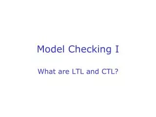
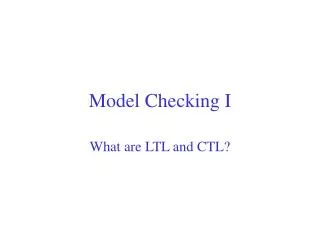
Model Checking I. What are LTL and CTL?. dack. and. or. q0. dreq. q0bar. and. View circuit as a transition system. (dreq, q0, dack) (dreq’, q0’, dack’) q0’ = dreq and dack’ = dreq & (q0 + ( q0 & dack)). dack. and. or. D. q0. dreq. D. and. dreq.

Model Checking I
E N D
Presentation Transcript
Model Checking I What are LTL and CTL?
dack and or q0 dreq q0bar and
View circuit as a transition system (dreq, q0, dack) (dreq’, q0’, dack’) q0’ = dreq and dack’ = dreq & (q0 + (q0 & dack))
dack and or D q0 dreq D and
dreq q0 q0’ dack’ dack
Idea Transition system + special temporal logic + automatic checking algorithm
Exercise (from example circuit) (dreq, q0, dack) (dreq’, dreq, dreq & (q0 + (q0 & dack))) Draw state transition diagram Q: How many states for a start?
Hint (partial answer) 000 100 110 111 001 101 010 011
Question 000 100 110 111 001 101 010 011 Q: how many arrows should there be out of each state? Why so?
Exercise 000 100 110 111 001 101 010 011 Complete the diagram Write down the corresponding binary relation as a set of pairs of states
Another view computation tree from a state 111
111 011 111 • 011 000 100 111 011 000 100 000 100 010 110 Unwinding further . . .
s Possible behaviours from state s Transition relation R . . . Relation vs. Function?
s path = possible run of the system Transition relation R . . .
Points to note Transition system models circuit behaviour We chose the tick of the transition system to be the same as one clock cycle. Gates have zero delay – a very standard choice for synchronous circuits Could have had a finer degree of modelling of time (with delays in gates). Choices here determine what properties can be analysed Model checker starts with transition system. It doesn’t matter where it came from
G(p -> F q) yes property MC algorithm no p p q q counterexample finite-statemodel Model Checking (Ken McMillan)
Netlist dack and or D 1 q0 dreq D 0 and
input to SMV model checker MODULE main VAR w1 : boolean; VAR w2 : boolean; VAR w3 : boolean; VAR w4 : boolean; VAR w5 : boolean; VAR i0 : boolean; VAR w6 : boolean; VAR w7 : boolean; VAR w8 : boolean; VAR w9 : boolean; VAR w10 : boolean; DEFINE w4 := 0; DEFINE w5 := i0; ASSIGN init(w3) := w4; ASSIGN next(w3) := w5; DEFINE w7 := !(w3); DEFINE w9 := 1; DEFINE w10 := w5 & w6; ASSIGN init(w8) := w9; ASSIGN next(w8) := w10; DEFINE w6 := w7 & w8; DEFINE w2 := w3 | w6; MC builds internal representation of transition system
Transition system M S set of states (finite) R binary relation on states assumed total, each state has at least one arrow out A set of atomic formulas L function A set of states in which A holds Lars backwards finite Kripke structre
Path in M Infinite sequence of states π = s0 s1 s2 ... st
Path in M s0 s1 s2 ... R (s0,s1) є R (s1,s2) є R etc
Read Another look at LTL model checking Clarke, Grumberg and Hamaguchi See course page
Properties Express desired behaviour over time using special logic LTL (linear temporal logic) CTL (computation tree logic) CTL* (more expressive logic with both . LTL and CTL as subsets)
CTL* path quantifers A “for all computation paths” E “for some computation path” can prefix assertions made from Linear operators G “globally=always” F “sometimes” X “nexttime” U “until” about a path
CTL* formulas (syntax) path formulas f ::= s | f | f1 f2 | X f | f1 U f2 state formulas (about an individual state) s ::= a | s | s1 s2 | E f atomic formulas
Build up from core A f E f F f true U f G f F f
Example G (req -> F ack)
Example G (req -> F ack) A request will eventually lead to an acknowledgement liveness linear
Example (Gordon) It is possible to get to a state where Started holds but Ready does not
Example (Gordon) It is possible to get to a state where Started holds but Ready does not E (F (Started & Ready))
Semantics M = (L,A,R,S) M, s ff holds at state s in M (and omit M if it is clear which M we are talking about) M, πg g holds for path π in M
Semantics Back to syntax and write down each case s a a in L(s) (atomic) s f not (s f) s f1 f2 s f1 or s f2 s E (g) Exists π. head(π) = sandπ g
Semantics πf s f and head(π) = s π g not(π g) π g1 g2 π g1 orπ g2
Semantics π X gtail(π) g πg1 U g2 Exists k ≥ 0. drop kπ g2 and Forall 0 ≤ j < k. drop j π g1 (note: I mean tail in the Haskell sense)
CTL Branching time (remember upside-down tree) Restrict path formulas (compare with CTL*) f ::= f | s1s2 | X s | s1 U s2 state formulas Linear time ops (X,U,F,G) must be wrapped up in a path quantifier (A,E).
Back to CTL* formulas (syntax) path formulas f ::= s | f | f1 f2 | X f | f1 U f2 state formulas (about an individual state) s ::= a | s | s1 s2 | E f atomic formulas
CTL Another view is that we just have the combined operators AU, AX, AF, AG and EU, EX, EF, EG and only need to think about state formulas A operators for necessity E operators for possibility
f :: = atomic | f Allimmediate successors | AX f Someimmediate succesor | EX f Allpaths always | AG f Somepath always | EG f Allpaths eventually | AF f Somepath eventually | EF f | f1 & f2 | A (f1 U f2) | E (f1 U f2)
Examples (Gordon) It is possible to get to a state where Started holds but Ready does not
Examples (Gordon) It is possible to get to a state where Started holds but Ready does not EF (Started & Ready)
Examples (Gordon) If a request Req occurs, then it will eventually be acknowledged by Ack
Examples (Gordon) If a request Req occurs, then it will eventually be acknowledged by Ack AG (Req => AF Ack)
Examples (Gordon) If a request Req occurs, then it continues to hold, until it is eventually acknowledged
Examples (Gordon) If a request Req occurs, then it continues to hold, until it is eventually acknowledged AG (Req => A [Req U Ack])
Exercise Draw computation trees illustrating AX f and EX f
Exercise Draw computation trees illustrating AG, EG, AF and EF (See nice pictures from Pistore and Roveri)
LTL LTL formula is of form A f where f is a path formula with subformulas that are atomic (and then, as usual, have E f = A f etc) Restrict path formulas (compare with CTL*) f ::= a | f | f1 f2 | X f | f1 U f2
Back to CTL* formulas (syntax) path formulas f ::= s | f | f1 f2 | X f | f1 U f2 state formulas (about an individual state) s ::= a | s | s1 s2 | E f atomic formulas
LTL It is the restricted path formulas that we think of as LTL specifications (See P&R again) G(critical1 & critical2) mutex FG initialised stays initialised once . Initialised GF myMove myMove will always eventually hold G (req => F ack) request acknowledge pattern
Not possible to express in LTL AG EF start Regardless of what state the program enters, there exists a computation leading back to the start state