Download
1 / 45
470 likes | 764 Vues
Multivariate Analysis. One-way ANOVA. Tests the difference in the means of 2 or more nominal groups E.g., High vs. Medium vs. Low exposure Can be used with more than one IV Two-way ANOVA, Three-way ANOVA etc. ANOVA. _______-way ANOVA Number refers to the number of IVs

E N D
One-way ANOVA • Tests the difference in the means of 2 or more nominal groups • E.g., High vs. Medium vs. Low exposure • Can be used with more than one IV • Two-way ANOVA, Three-way ANOVA etc.
ANOVA • _______-way ANOVA • Number refers to the number of IVs • Tests whether there are differences in the means of IV groups • E.g.: • Experimental vs. control group • Women vs. Men • High vs. Medium vs. Low exposure
Logic of ANOVA • Variance partitioned into: • 1. Systematic variance: • the result of the influence of the Ivs • 2. Error variance: • the result of unknown factors • Variation in scores partitions the variance into two parts by calculating the “sum of squares”: • 1. Between groups variation (systematic) • 2. Within groups variation (error) • SS total = SS between + SS within
Significant and Non-significant Differences Non-significant: Within > Between Significant: Between > Within
Partitioning the Variance Comparisons • Total variation = score – grand mean • Between variation = group mean – grand mean • Within variation = score – group mean • Deviation is taken, then squared, then summed across cases • Hence the term “Sum of squares” (SS)
One-way ANOVA example Total SS (deviation from grand mean) Group A Group B Group C 49 56 54 52 57 52 52 57 56 53 60 50 49 60 53 Mean = 51 58 53 Grand mean = 54
One-way ANOVA example Total SS (deviation from grand mean) Group A Group B Group C -5 25 2 4 0 0 -2 4 3 9 -2 4 -2 4 3 9 2 4 -1 1 6 36 -4 16 -5 25 6 36 -1 1 Sum of squares = 59 + 94 + 25 = 178
One-way ANOVA example Between SS (group mean – grand mean) A B C Group means 51 58 53 Group deviation from grand mean -3 4 -1 Squared deviation 9 16 1 n(squared deviation) 45 80 5 Between SS = 45 + 80 + 5 = 130 Grand mean = 54
One-way ANOVA example Within SS (score - group mean) A B C 51 58 53 Deviation from group means -2 -2 1 1 -1 -1 1 -1 3 2 2 -3 -2 2 0 Squared deviations 4 4 1 1 1 1 1 1 9 4 4 9 4 4 0 Within SS = 14 + 14 + 20 = 48
The F equation for ANOVA F = Between groups sum of squares/(k-1) Within groups sum of squares/(N-k) N = total number of subjects k = number of groups Numerator = Mean square between groups Denominator = Mean square within groups
Significance of F F-critical is 3.89 (2,12 df) F observed 16.25 > F critical 3.89 Groups are significantly different -T-tests could then be run to determine which groups are significantly different from which other groups
Two-way ANOVA • ANOVA compares: • Between and within groups variance • Adds a second IV to one-way ANOVA • 2 IV and 1 DV • Analyzes significance of: • Main effects of each IV • Interaction effect of the IVs
Graphs of potential outcomes • No main effects or interactions • Main effects of color only • Main effects for motion only • Main effects for color and motion • Interactions
Graphs A R O U S A L x Motion * Still Color B&W
No main effects for interactions A R O U S A L x Motion * Still Color B&W
No main effects for interactions A R O U S A L x Motion x x * Still * * Color B&W
Main effects for color only A R O U S A L x Motion * Still Color B&W
Main effects for color only A R O U S A L * x x Motion * Still * x Color B&W
Main effects for motion only A R O U S A L x Motion * Still Color B&W
Main effects for motion only A R O U S A L x x x Motion * Still * * Color B&W
Main effects for color and motion A R O U S A L x Motion * Still Color B&W
Main effects for color and motion A R O U S A L x x Motion x * Still * * Color B&W
Transverse interaction A R O U S A L x Motion * Still Color B&W
Transverse interaction A R O U S A L x * x Motion * Still x * Color B&W
Interaction—color only makes a difference for motion A R O U S A L x Motion * Still Color B&W
Interaction—color only makes a difference for motion A R O U S A L x x Motion * Still * x * Color B&W
Partitioning the variance for Two-way ANOVA Total variation = Main effect variable 1 + Main effect variable 2 + Interaction + Residual (within)
Summary Table for Two-way ANOVA SourceSSdfMSF Main effect 1 Main effect 2 Interaction Within Total
Scatter Plot of Price and Attendance • Price is the average seat price for a single regular season game in today’s dollars • Attendance is total annual attendance and is in millions of people per annum.
Is there a relation there? • Lets use linear regression to find out, that is • Let’s fit a straight line to the data. • But aren’t there lots of straight lines that could fit? • Yes!
Desirable Properties • We would like the “closest” line, that is the one that minimizes the error • The idea here is that there is actually a relation, but there is also noise. We would like to make sure the noise (i.e., the deviation from the postulated straight line) to be as small as possible. • We would like the error (or noise) to be unrelated to the independent variable (in this case price). • If it were, it would not be noise --- right!
Scatter Plot of Price and Attendance • Price is the average seat price for a single regular season game in today’s dollars • Attendance is total annual attendance and is in millions of people per annum.
Simple Regression The simple linear regression MODEL is: y = 0 + 1x + describes how y is related to x 0 and 1 are called parameters of the model. is a random variable called the error term. x y e
Simple Regression • Graph of the regression equation is a straight line. • β0 is the population y-intercept of the regression line. • β1 is the population slope of the regression line. • E(y) is the expected value of y for a given x value
Simple Regression E(y) Regression line Intercept 0 Slope 1 is positive x
Simple Regression E(y) Regression line Intercept 0 Slope 1 is 0 x
Regression Modeling Steps • 1. Hypothesize Deterministic Components • 2. Estimate Unknown Model Parameters • 3. Specify Probability Distribution of Random Error Term • Estimate Standard Deviation of Error • 4. Evaluate Model • 5. Use Model for Prediction & Estimation
Linear Multiple Regression Model • 1. Relationship between 1 dependent & 2 or more independent variables is a linear function Population Y-intercept Population slopes Random error Dependent (response) variable Independent (explanatory) variables
Multiple Regression Model Multivariate model