Download
1 / 32
340 likes | 567 Vues
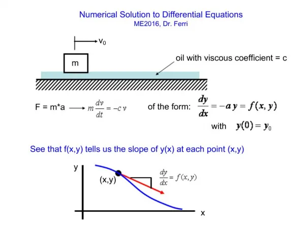
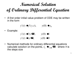
Numerical solution of Differential and Integral Equations. PSCi702 October 19, 2005. Differential Equations. Equations where the dependent variable appears as well as one or more of its derivatives. The highest derivative present determines the order of differential equation.

E N D
Numerical solution of Differential and Integral Equations PSCi702 October 19, 2005
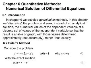
Differential Equations • Equations where the dependent variable appears as well as one or more of its derivatives. • The highest derivative present determines the order of differential equation. • The highest power of the dependent variable or its derivative sets the degree of the differential equation.
Differential Equations • Y’-Y=0 (1st order) • Y’(t)-Y(t)=exp(t) (1st order) • Y’(t)-Y(t)=t2 (1st order) • Y’’+Y’-2Y=0 (2nd order) • Y’’’+Y’’-2Y=0 (3rd order) • Y’+Y2=0 ( 2nd degree, 1st order) • Y’’(t)+(Y’(t)-Y(t))2 =t ( 2nd degree, 2nd order)
Differential Equations • Higher order equations can be reduced to a system of first order equations.
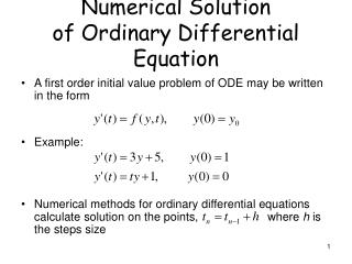
Differential Equations • When solving differential equations, the final answer has a constant of integration in it. • If all the constants of integrations are specified at the same place, they are then called initial values and the solution is called initial value problem. • If the initial values are not given at the same place and are specified at different locations, then the solution to the problem is called boundary value problem.
Solution to Differential Equations • Start the solution at the value of the independent variable for which the solution is equal to initial values. • Proceed step by step by changing the independent variable and obtaining solution across the required range. • Since most methods use local polynomial approximation methods, stability becomes an issue.
One Step Methods • Picard’s Method
Example Use Picard iteration to find the solution of
Example • The exact solution is:
Runge-Kutta • The method doesn’t rely on polynomial approximation. • Solution can be presented by a finite taylor series of the form:
Error Estimate • If solution is monotonically increasing, then the error is increasing as well due to truncation. • In oscillatory solutions, the truncation error introduces a phase shift. • The general accuracy can not be arbitrarily increased by decreasing the step size. While it will reduce the truncation error, it will increase the effects of round-off error.
Predictor-Corrector Method • By using the solution at n points, we can fit an (n-1) degree polynomial. • The predictor part extrapolates the solution over some finite range h based on the information at prior points and inherently unstable. • The corrector part makes correction at the end of the interval based on some prior information.
Systems of Differential Equations • In vector form: • Where consists of elements which are functions of dependent variables yi,n and xn. • A set of basis solutions is simply a set of solutions, which are linearly independent. • Consider a set of m linear first order differential equations where k values of the dependent variables are specified at x0 and (m-k) values corresponding to the remaining dependent variables are specified at xn.
Systems of Differential Equations • solve (m-k) initial value problems starting at x0 and specifying (m-k) independent, sets of missing initial values so that the initial value problems are uniquely determined. Let us denote the missing set of initial values at x0 by
The columns of are just the individual vectors • Matix A will have to be diagonal to always produce • So one can choose • So the missing initial values will be
Integral Equations • Equations can be written where the dependent variable appears under an integral as well as alone. • Such equations are the analogue of the differential equations and are called integral equations. • It is often possible to turn a differential equation into an integral equation which may make the problem easier to numerically solve.
Integral Equations • The parameter K(x,t) appearing in the integrand is known as the kernel of the integral equation. • Its form is crucial in determining the nature of the solution. Certainly one can have homogeneous or inhomogeneous integral equations depending on whether or not F(x) is zero. Of the two classes, the Fredholm are generally easier to solve.