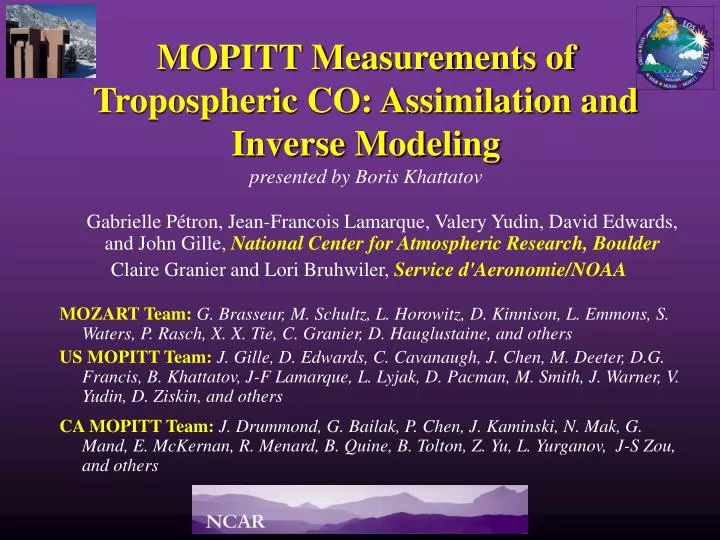
MOPITT Measurements of Tropospheric CO: Assimilation and Inverse Modeling presented by Boris Khattatov

1. MOPITT Measurements of Tropospheric CO: Assimilation and Inverse Modeling presented by Boris Khattatov Gabrielle Pétron, Jean-Francois Lamarque, Valery Yudin, David Edwards, and John Gille, National Center for Atmospheric Research, Boulder Claire Granier and Lori Bruhwiler,Service d'Aeronomie/NOAA MOZART Team:G. Brasseur, M. Schultz, L. Horowitz, D. Kinnison, L. Emmons, S. Waters, P. Rasch, X. X. Tie, C. Granier, D. Hauglustaine, and others US MOPITT Team:J. Gille, D. Edwards, C. Cavanaugh, J. Chen, M. Deeter, D.G. Francis, B. Khattatov, J-F Lamarque, L. Lyjak, D. Pacman, M. Smith, J. Warner, V. Yudin, D. Ziskin, and others CA MOPITT Team:J. Drummond, G. Bailak, P. Chen, J. Kaminski, N. Mak, G. Mand, E. McKernan, R. Menard, B. Quine, B. Tolton, Z. Yu, L. Yurganov, J-S Zou, and others

2. Introduction The goal of this research project is to study global distributions and derive poorly known surface sources of CO from MOPITT data. This is done via assimilation of MOPITT data and inverse modeling of CO emissions in the MOZART 2 model.

3. Data Assimilation Mathematical basis of data assimilation is estimation or inverse problem theory: “People were naked worms; yet they had an internal model of the world. In the course of time this model has been updated many times, following the development of new experimental possibilities or their intellect. Sometimes the updating has been qualitative, sometimes it has been quantitative. Inverse problem theory describes rules human beings should use for quantitative updating” Albert Tarantola, Inverse Problem Theory Andrey Kolmogorov Norbert Weiner

4. 1-D Estimation To optimally combine two pieces of information one has to know their uncertainties (errors).

5. Multiple Dimensions • x is a vector, e.g., • concentrations of several chemicals at the same location • concentrations of the same chemical at different locations If we know that element xicorrelates with xj, we can infer information about xjfrom measurements of xi => error covariance matrices

6. Dynamic estimation Let’s assume we have a time dependent predictive modelM: x(t+Dt) = M[ x(t) ] The model tries to predict quantity x, which can be a scalar or a vector. Model simulations have uncertaintysxassociated with them Let’s also assume that there exist independent observations of quantity y, which is related to x via: y = H[ x ] The uncertainty of measurements of y issy

7. The problem Model: Observations: Observational operator: Problem:find the “best” x, which inverts for a given y allowing for observation errors and other prior information y = M(x) z z = H(y) z = H(M(x))

8. 0-D Example (a scalar x) Let’s assume that we measure x directly, i.e., H = I x time

9. 0-D Example (a scalar x) x time

10. 0-D Example (a scalar x) If we use optimal estimates of x as initial conditions for model integration we can improve model predictive skills. To do this systematically we need to be able to computethe time evolution of errors in the model x time

11. X3 Z3 H X2 Z2 X1 Z1 Mathematical Basis • Arrange observations in vector z, Nz~102-104 • Arrange model variables in vector x, Nx~104-106 • Define “observational” operator H: transformation from model variables to observations (interpolation) • Invert (in the statistical sense) z = H(M(x)) observation space ~ 104 dimensions model space ~ 106 dimensions

12. The problem Formally, findx that minimizes B and O are the forecast and observational error covariances J(x) = [z -H(M(x))]TO-1[z-H(M(x))] + [x - xa]TBa-1[x-xa]

13. Evolution of the PDF is governed by a differential equation (Fokker-Kolmogorov) which is impossible to solve in most practical cases Therefore, simplifications are necessary

14. Approximations • PDFs are Gaussian: • Bis the covariance matrix PDF(x) ~ e-0.5(x-<x>)TB-1(x-<x>) B = <(x-<x>)(x-<x>)T>

15. Approximations . Model can be linearized for small perturbations: H(M[x(t) +x(t)]) ≈ H(M[x(t)]) + Lx(t) dx(t + t) dH(M(x)) L = = dx(t) dx Lis the linearization matrix

16. Linearization For photochemically active gases, like CO, the relationship y=H(x) between x and y is non-linear In order to solve the problem one needs to linearize the model and use iterative techniques for finding the solution We assume that the model can be linearized with respect to the emissions for small perturbations: H[x +x] ≈ H[x] + Lx dH dy(t + t) L = = dx(t) dx

17. Linearization So, H can be approximated using the linearization matrix. L can be obtained 1. Using finite differences -- by running the model N times (where N is the number of emission sources), once for each source while all but one source are set to zero., i.e., L~ Dy/Dx 2. By differentiating the computer code of the model, i.e., developing computer code that calculates matrix L for given x and y

18. Linearization 1. Linearization via finite differences (L~ Dy/Dx): Pros: straightforward to construct, easy to change models Cons: takes a lot of CPU time 2. Linearization by differentiating the computer code of the model: Pros: Small CPU requirements Cons: complicated to construct, hard to switch models

19. The Solution x = xa + K(z - H(M(xa))) K = BaLT(LBaLT + O)-1 B = Ba - BaLT(LBaLT + O)-1LBa

20. Chemistry-Transport Model Chemistry and Transport parameterizations Final 3-D CO distribution y(t+Dt) y(t + t) = M[y(t),x] Initial 3-D CO distribution, y(t) x

21. 2n n n n n 2n 2n x2 x z2 y2 t z y Chemistry-Transport ModelBasic Equation + u +v +w = D + + + P - L(n) n – pollutant concentration u,v,w – wind vector components D – diffusion coefficient P – production of pollutant L – loss of pollutant

22. n n n n 2n 2n 2n y2 x2 x y z t z2 + u +v +w = D + + Chemistry-Transport Model1. Emissions + P - L(n)

23. 2n n 2n 2n t x2 y2 z2 n n n y z x Chemistry-Transport Model2. Advection +u +v +w = D + + + P- L(n)

24. 2n n 2n 2n t x2 y2 z2 n n n y z x Chemistry-Transport Model3. Convection +u +v +w = D + + + P- L(n)

25. n n n n z y t x 2n 2n 2n y2 x2 z2 Chemistry-Transport Model4. (Turbulent) Diffusion +u +v +w =D + + + P- L(n)

26. n n n n 2n 2n 2n y2 x2 x y z t z2 + u +v +w = D + + Chemistry-Transport Model5. Chemistry + P - L(n)

27. MOZART2 Model • 3-D global CTM MOZART 2 • 5° longitude by 5° latitude (T21) and higher (T42, T63) • 28-60 levels • Tropospheric chemistry, ~50 species • ECMWF or NCEP dynamics • Developed at NCAR and then at Max Plank

28. MOPITT Mission TheMeasurement Of Pollution In The Troposphere mission is a joint CSA and NASA project. U. of Toronto leads the Canadian effort to contribute the instrument. NCAR leads the US effort do develop and apply data processing algorithms and provide science support During the 5 year mission, MOPITT will provide the first long term, global measurements of carbon monoxide (CO) & methane (CH4) levels in the troposphere.

29. MOPITT Mission The field-of-view of MOPITT is 22 x 22km and it views four fields simultaneously. The field of view is also continuously scanned through a swath about 600 km wide as the instrument moves along the orbit.

30. This Study Used Preliminary MOPITT Data The MOPITT instrument and the measurement technique are unique: lessons are being learned for the first time in both instrument operation and data processing The US and Canadian MOPITT Teams work very hard on identifying and removing potential problems in the retrieved CO data and recently succeeded in delivering first data to NASA The released data (internal version V4.6.2) is considered beta; individual profiles might contain noise that needs to be understood better This study used V4.3.1 – all data were binned in 5x5 degree bins

31. Instantaneous Isosurface of CO, MOZART 2

32. MOPITT Data

33. Analysis Model Assimilation of MOPITT CO

34. Instantaneous Isosurface of CO, MOPITT Assimilation

35. Isosurface of CO, MOZART2

36. CO, March-December 2000

37. Inverse Modeling yo ym MOPITT MOZART The discrepancies between observations and model results can be used to optimize poorly known parameters in the model – e.g., surface emissions.

38. March 2000 : Total column of CO MOZART2 (top) and MOPITT (bottom) MAR MOZART2, CO-column, scale=1.e17 60 40 20 0 Latitude -20 -40 -60 -100 0 100 MAR MOPITT, CO-column, scale=1.e17 60 40 20 0 Latitude -20 -40 -60 -100 0 100 Longitude

39. July 2000: Total column of CO MOZART2 (top) and MOPITT (bottom) JUL MOZART2, CO-column, scale=1.e17 60 40 20 0 Latitude -20 -40 -60 -100 0 100 JUL MOPITT, CO-column, scale=1.e17 60 40 20 0 Latitude -20 -40 -60 -100 0 100 Longitude

40. CO “colors”, day 2

41. CO “colors”, day 65

42. CO “colors”, day 85

43. CO “colors”, 4 months

44. MOPITT CO Inversion We performed first inversion experiments using a finite-differences constructed linearization of the MOZART 2 model MOPITT August observations of CO at 500mb were used to constrain model surface emissions of CO for August 2000

45. a priori CO emissions, August 2000

46. CO MOPITT inversion August 2000

47. CO MOPITT inversion, August 2000