Download

1 / 23
240 likes | 509 Vues
Image Processing. Image processing. Once we have an image in a digital form we can process it in the computer . We apply a “filter” and recalculate the pixel values of the processed image. We will look at the application of filters to sharpen and soften (make less sharp) the image.

E N D
Image processing • Once we have an image in a digital form we can process it in the computer. • We apply a “filter” and recalculate the pixel values of the processed image. • We will look at the application of filters to sharpen and soften (make less sharp) the image.
Filters or Kernals • Our filters take the form of a small matrix or vector which we place (in turn ) over the image at each pixel position. • Typically our filters are symmetrical 3 x 3 matrices. • We use a process called convolution to apply the filter to the image.
Convolution • Convolution is the process of multiplying each element of our filter by the pixel values of the image that the filter covers and adding the products. • We can describe the result as “the original image convolved with the filter”. • conv2 is a Matlab function which can do this. Strictly what is described above is not a convolution but a correlation, however if our filters are symmetric the result is the same.
-1 -1 0 0 0 0 -1 -1 -1 -1 4 4 -1 -1 0 0 0 0 Convolution and filters Filter 56 56 56 56 56 56 59 89 15 Image sample set 1 5 4 2 3 7 9 4 5
Convolution and filters 56 56 56 56 56 56 59 89 15 Image sample set 1 -1 0 5 0 4 -1 2 3 7 -1 4 9 -1 4 5 0 0
Convolution and filters 1 -1 0 5 0 4 2 -1 3 7 -1 4 4 5 9 -1 4 5 3 7 0 0 9 4 5 So the value of 3 in the centre of the original image is replaced with –5 on the convolved image.
Image softening • If we make all the elements of the filter equal to one ninth, then the convolution value will be the average of all the elements “covered” by the filter. • It is the same as adding all the 9 values together and dividing by nine.
Image softening • The following block of image samples represents a sharp vertical edge as pixel values suddenly change from 0 (black) to 255 (white). • We will attempt to smooth it (make it less sharp). Sample Block
Image softening • Consider the operation of the averaging filter on the block of image samples. Filter Sample Block
Image softening • As we “run” the filter over the centre of the sample block. The following changes will take place. See next slide. Filter Sample Block
Image softening • The zeros in the 4th column are replaced with 85, since:
Image softening • Similarly as we perform the convolution of the filter with the rest of the centre of the sample block we get:
Image softening • The resultant convolution (image) no longer has a sharp edge, but a more gradual one.
Image softening • That’s the theory; lets try it. for i=1:256 grey(i, 1:3)=(i-1)/255 end colormap(grey) myedge=zeros(5, 8) myedge(:, 5:8)=255 filt=ones(3,3)/9 image(myedge) myconv=conv2(myedge,filt, 'valid') image(myconv)
Softening an image im=imread(‘urban.bmp'); smooth=[ 1 1 1; 1 1 1; 1 1 1]/9 % convolve all colours smoothim(:,:,1)=conv2(im(:,:,1),smooth); smoothim(:,:,2)=conv2(im(:,:,2),smooth); smoothim(:,:,3)=conv2(im(:,:,3),smooth); image(im) figure image(uint8(smoothim))
Image sharpening • It is easier to see this in one dimension initially. • Consider some neighbouring pixels that are not sharp. • If they are not sharp there will be no abrupt change in value between them. • If we can cause an a more abrupt change in value between neighbouring pixels, we will sharpen the image.
Image sharpening • It is easier to see this in one dimension initially. • Consider some neighbouring pixels that are not sharp. • If they are not sharp there will be no abrupt change in value between them. • If we can cause an a more abrupt change in value between neighbouring pixels, we will sharpen the image.
Image sharpening • The idea is to generate artificial sharp edges at the points of differing neighbouring pixels and then add these edges to the original image. • The following diagram shows the variation in brightness values for: • (a) A perfect (sharp) edge. • (b) A blurred edge. • (c) The artificial correction to be added. • (d) The corrected (enhaced) edge.
Image sharpening 200 (a) 100 200 (b) 150 100 50 (c) -50 250 200 150 (d) 100 50
-1 0 0 -1 -1 4 -1 0 0 -1 -1 2 2 Image sharpening • What kernal (filter) will (when convolved with the image) generate the correction waveform (c) ? • In one dimension • Check it. • It produces zero for flat fields, but a negative and positive edge at edges • In two dimensions
-1 0 -1 0 0 0 0 0 0 0 0 0 -1 0 -1 0 0 -1 0 -1 1 4 5 1 -1 0 -1 0 0 0 0 0 0 0 0 0 Image sharpening • We need to produce a kernal which will add the artificial edges and the original together. • The original will be produced if we only have a one (1) in the centre of the a convolution kernal. Check it. • Add this to the edge generator + =
Sharpening an Image im=imread(‘urban.bmp'); sharp=[ 0 –1 0; -1 5 –1; 0 –1 0] % convolve all colours sharpim(:,:,1)=conv2(im(:,:,1),sharp); sharpim(:,:,2)=conv2(im(:,:,2),sharp); sharpim(:,:,3)=conv2(im(:,:,3),sharp); image(im) figure image(uint8(sharpim))