Download
1 / 30
300 likes | 403 Vues
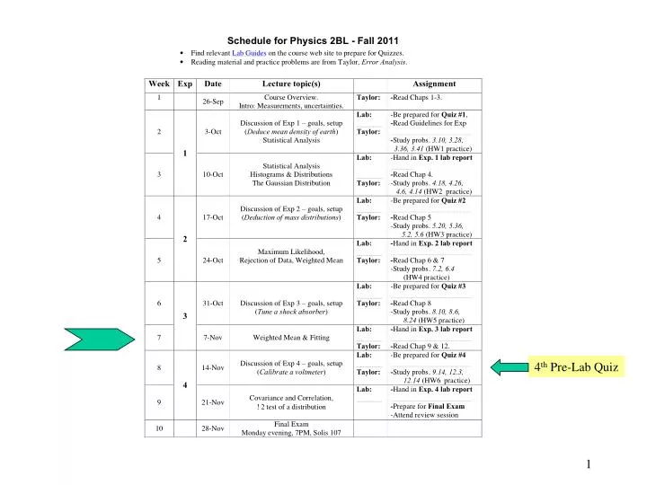
4 th Pre-Lab Quiz. Today ’ s Lecture:. Issues in Experiment #3 thanksgiving logistics… Reminder from previous lectures: Maximum likelihood and weighted mean Main topics today: Fitting c 2 Test of a distribution, goodness of fit. Logistics.

E N D
Today’s Lecture: • Issues in Experiment #3 • thanksgiving logistics… • Reminder from previous lectures: • Maximum likelihood and weighted mean Main topics today: • Fitting • c2 Test of a distribution, goodness of fit
Logistics • During Thanksgiving week A05,A07,A08 need to be rescheduled: Make-up sessions on Monday Nov. 21st Thanksgiving week is the last lab of the quarter The reports are due at the lab, during that week!
Maximum Likelihood Principle Recap from last Lecture The best estimates for X and sof N observed measurements, xi are those for which Prob X,(xi) is maximum.
Recall the probability density for measurements of some quantity x (distributed as a Gaussian with mean X and standard deviation ) Normal distribution is one example of P(x). Now, lets make repeated measurements of x to help reduce our errors. We define the Likelihood as the product of the probabilities. The larger L, the more likely a set of measurements is. The Principle of Maximum Likelihood Agreed that L is a Probability The best estimate for the parameters of P(x) are those that maximize L. We used this to prove the definitions of mean and SDOM
Weighted Averages We can use maximum Likelihood (c2) to average measurements with different errors. We derived the result that: Using error propagation, we can determine the error on the weighted mean: What does this give in the limit where all errors are equal?
Example of Weighted Average three measurements of a resistance what is the best estimate for R ?
Linear Fit • Determine A and B by minimizing the square of the deviations between your measurements and the “theory”. “Theory” Measurements
Fitting Data • We often fit data using a maximum likelihood method to determine parameters. • For errors which are “Normal”, we can just minimize the c2. • We will use this method to fit straight lines to data. • More complex functions can be fit the same way. To determine a straight line we need 2 parameters. How do we get at least 2 equations?
S [yj-(A+Bxj)] LINEAR FIT: y(x) = A + Bx true value 2 minimize y4-(A+Bx4) y3-(A+Bx3) Assumptions: dxj << dyj ; dxj = 0 yj – normally distributed sj: same for all yj
S [yj-(A+Bxj)] 2 Best estimates of A&B max Prob(y1…yN) min LINEAR FIT: y(x) = A + Bx
minimize: S [yj-(A+Bxj)] Sometime denote: 2 LINEAR FIT: y(x) = A + Bx To determine A & B need to
Least‐Squares Fitting: General Remarks • In practice,you will usually use a software package to compute the least‐squares fit to your data. • Our goal here is for you to understand HOW these formulae were derived, but it is not necessary to memorize them. • We will assume that errors are only significant in y. This is not always the case. • These procedures can be generalized to fitting polynomials, exponential functions and functions involving more than two variables (section 8.6 in Taylor).
Deducing Errors • As in the case of experiment 2, sometimes we can’t estimate the errors too well before-hand. • In such cases we compared many measurements to the mean and computed the RMS. • In this case we will compare to deviations from a line • 2 Dimension “extension”. Note that now we use (n-2) because we have fit 2 parameters. Where did we use (n-1)?
Motivation for the (n-2) • Averages (1 parameter) • no deviations from one point • “reduced” deviations from two points • Straight lines (2 parameters) • no deviations from two points • “reduced” deviations form three points
Uncertainties in y, A, and B uncertainty in the measurement of y uncertainties in the constants A and B given by error propagation in terms of uncertainties in y1, … , yN Where
Reminder of LSQ Assumptions • All data points have Gaussian errors. • The errors on different points are not correlated. Maximum Likelihood Method is more general than LSQ. Maximum Likelihood Method can (in principle) be applied to any situation. In real life, it is often quite difficult.
Summary - Fitting • You have a set of measurements and a hypothesis that relates them. • The hypothesis has some unknown parameters that you want to determine. • You “fit” for the parameters by maximizing the odds of all measurements being consistent with your hypothesis. Next: • Evaluate your fit based on the goodness of fit.
c2TEST for FIT Roughly speaking: - O(N) it’s a good fit - >>N it’s a Bad fit How good is the agreement between theory and data?
c2TEST for FIT Define: Reduced chi2 # of degrees of freedom d = N - c # of data points # of parameters calculated from data # of constraints
The Chi-square Test • We have used c2 minimization to fit data. • We can also use the value of c2to determine if the data fit the hypothesis. • On average, the c2 value is about one per degree of freedom. • The number of degrees of freedom is the number of measurements minus the number of fit parameters. • We will use the c2 per degree of freedom to compute a probability that the data are consistent with the hypothesis. (table D) • This probability of c2 is like the confidence level.
disagreement is “significant” if ProbN(c2 ≥ c02) is less than 5 % disagreement is “highly significant” if ProbN(c2 ≥ c02) is less than 1 % reject the expected distribution Probability of Chi-square quantitative measure of agreement between observed data and their expected distribution probability of obtaining a value of c2 greater or equal to c02 , assuming the measurements are governed by the expected distribution
The Chi-Squared Test for a distribution • You take N measurements of some parameter x which you believe should be distributed in a certain way (e.g., based on some hypothesis). • You divide them into n bins (k=1,2,...,n) and count the number of observations that fall into each bin (Ok). • You also calculate the expected number of measurements (Ek), in the same bins, based on some hypothesis. • Calculate: • Ifχ2<n, then the agreement between the observed and expected distributions is acceptable. • Ifχ2>>n, there is significant disagreement.
Example: Application of c2Test Die is tossed 600 times Expectation: each face has same likelihood of showing up v 1 2 3 4 5 6 _ Verification of expectation by computing the obs 91 137 111 87 80 94 c2 exp 100 100 100 100 100 100 D2 81 1369 121 169 400 36 s 10 10 10 10 10 10 c 2 This term is the squared difference between observation and expectation. In computation of c2 the D2 term is divided by expectation. s is square root of expectation (Ey = sy2) 0.81 13.7 1.21 1.69 4.0 0.36 i Total 21.76 c2 ndof 5 c2 reduced 4.35
Application of c2Test: Use Table D Just calculated: Totalc221.77 ndof5 Reducedc24.35 Die is loaded at 99.9% Confidence Level
Degrees of Freedom - revisited • Number of degrees of freedom, d = number of observations, Ok, minus the number of parameters computed from the data and used in the calculation. • d=n‐c, • Where c is the number of parameters that were calculated in order to compute the expected numbers, Ek. • It can be shown that the expected average value ofχ2 is d. • Therefore, we defined “reduced chi‐squared”: • If reduced chi-squared is <1, there is no reason to doubt the expected distribution.
Example • We measure the height of every student in the class (say of 50).We compute a mean height, <h> with a standard deviation σh. Then we bin the measurements as follows: • Less than (<h>‐σh): 9 • Between (<h>‐σh) and <h>: 15 • Between <h> and (<h>+σh): 19 • More than (<h>+σh): 7 • Assuming the measurements are normally distributed: • What is the expected number of measurements in each bin? • What is the χ2? • Do you conclude that the students heights are distributed normally?
Solution From Table B: • Less than (<h>‐σh): 0.5 - 0.34 = 0.16 0.16*50= 8 • Between (<h>‐σh) and <h>: 0.34 0.34*50=17 • Between <h> and (<h>+σh): 0.34 0.34*50=17 • More than (<h>+σh): 0.5 - 0.34 = 0.16 0.16*50= 8 Ok 9 15 19 9 Ek 8 17 17 8 Finish it yourselves…
Next Lecture… • Introduction to Exp #4 • Reminder and examples: Testing for goodness of fit - c2