Download
1 / 27
280 likes | 448 Vues
Evaluation of Relational Operations. Why does a DBMS implements several algorithms for each algebra operation? What are query evaluation plans and how are they represented? Why is it important to find good evaluation plan for a query? How is this done in relational DBMS? .

E N D
Evaluation of Relational Operations • Why does a DBMS implements several algorithms for each • algebra operation? • What are query evaluation plans and how are they represented? • Why is it important to find good evaluation plan for a query? • How is this done in relational DBMS?
System Catalogs For each index: • name, structure (e.g., B+ tree) and search key fields For each relation( table ): • name, file name, file structure (e.g., Heap file) • attribute name and type, for each attribute • index name, for each index • integrity constraints For each view: • view name and definition Plus statistics, authorization, buffer pool size, Page size etc. • Catalogs are themselves stored as relations!
The following information is commonly stored Cordinality: (NTuples(R)) -#of tupelws for each table R Size: (NPages(R)) - # of pages Index Cordiality: (NKyes(I)) - # of distinct key values for each index I Index size: ( INPages(I)) - # of pages for each index I Index Height: ( IHeight(I)) - # of nonleaf levels Index Range: ( ILow(I) , and IHeigh(I) ) minimume and maximum value of present keys The Catalog also contains information about users, - account information's and authorizations
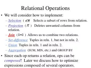
Relational Operations We will consider how to implement: • Selection ( ) Selects a subset of rows from relation. • Projection ( ) Deletes unwanted columns from relation. • Join ( ) Allows us to combine two relations. • Set-difference ( ) Tuples in reln. 1, but not in reln. 2. • Union ( ) Tuples in reln. 1 and in reln. 2. • Aggregation(SUM, MIN, etc.) and GROUP BY Since each op returns a relation, ops can be composed! After we cover the operations, we will discuss how to optimize queries formed by composing them.
Schema for Examples Sailors (sid: integer, sname: string, rating: integer, age: real) Reserves (sid: integer, bid: integer, day: dates, rname: string) Similar to old schema; rname added for variations. Reserves: Each tuple is 40 bytes long, 100 tuples per page, 1000 pages. Sailors: Each tuple is 50 bytes long, 80 tuples per page, 500 pages.
Three common techniques Indexing: If a selection or join condition is specified, use an index to examine just the tuples that satisfy the condition. Iteration: Examine all tuples in an input table, one after the other.( Some times we can examine index entries if the fields we are interested in are in index key ). Partitioning: by partitioning tuples on a sort key, we can often decompose an operation into a less expensive collection of operations on partitions. Sorting and Hashingare the common partitioning techniques
Access Path An access path as a way of retrieving tuples from a table and consists of either (1) file scan o (2) An index plus a matching selection condition. Intuitively an index matches a selection condition if the index can be used to retrieve just the tuples that satisfy the condition. A hash index matches a CFN selection if there is a term attribute = value in selection condition for each attr. In the index’s search key A tree index matches a CNF selection if there is a term of the form attribute op value for each attr in a prefix of the index’s key.
Examples of Access Paths If we have a hash index on search key <sname, bib, sid> then we can use the index to retrieve just the Seilors tuples with sname = ‘ Joy’ ^ bid = 5 ^ sid = 3 . In contrast, if the index were a B+ tree it would match sname = ‘ Joy’ ^ bid = 5 ^ sid = 3 and sname = ‘ Joy’ ^ bid = 5 However, it would not match bid = 5 ^ sid = 3 . What if we have an index on the search key <bid, sid> and the selection codition is sname = ‘ Joy’ ^ bid = 5 ^ sid = 3 ?
Selectivity of Access Pths The selectivity of an access path is the # of pages retrieved( index pages + data pages) if we use the access path to retrieve all desired tuples. The most selective access path is the one that retrieves the fewest pages. The fraction of tuples in the table that satisfy the given conjunct is called reduction factor. Example: Suppose we have a hash index H on Sailors with search key < sname, bid, sid> and we are given the selection codition sname = ‘ Joy’ ^ bid = 5 ^ sid = 3 . The fraction of pages satisfying the primary conjunct is Npages(H)/NKeys(H).
Algorithm for Relational Operations (Selection) The selection operator is simple retrieval of tuples from a table. For the selection of the form σR.attr op value (R)if there isindes on R.attr we have to scan R Size of result approximated as size of R * reduction factor; we will consider how to estimate reduction factors later. With no index, unsorted: Must essentially scan the whole relation; cost is M (#pages in R). With an index on selection attribute: Use index to find qualifying data entries, then retrieve corresponding data records. (Hash index useful only for equality selections.) SELECT * FROM Reserves R WHERE R.rname < ‘C%’
Using an Index for Selections Cost depends on #qualifying tuples, and clustering. • Cost of finding qualifying data entries (typically small) plus cost of retrieving records (could be large w/o clustering). • In example, assuming uniform distribution of names, about 10% of tuples qualify (100 pages, 10000 tuples). With a clustered index, cost is little more than 100 I/Os; if unclustered, upto 10000 I/Os! Important refinement for unclustered indexes: 1. Find qualifying data entries. 2. Sort the rid’s of the data records to be retrieved. 3. Fetch rids in order. This ensures that each data page is looked at just once (though # of such pages likely to be higher than with clustering).
Projection If duplications need not be eliminated , this can be accomplished by simple iteration on either the table or an index whose key is contains all necessary fields. If we have to eliminate the duplicates: let say we want to obtain < sid, bib> by projecting fro Reserves. We can first partition by scanning Reserves to obtain < sid, bid> pairs and than sort these pairs using < sid, bid > as sort key. Sorting is very important operation in database systems. Sorting a table typically requires two or three passes, each of which reads and writes entire table. Projection can be optimized by combining with sorting.
Sort-based approach is the standard; If an index on the relation contains all wanted attributes in its search key, can do index-onlyscan. • Apply projection techniques to data entries (much smaller!) If an ordered (i.e., tree) index contains all wanted attributes as prefix of search key, can do even better: • Retrieve data entries in order (index-only scan), discard unwanted fields, compare adjacent tuples to check for duplicates.
Joins Joins are expensive operations and very common. Consider the join of Reserves and Sailors with the Join condition R.sid = S.sid. Suppose that one of the tables, say Sailors has an index on the sid column. We can scan the Reserves and for each tuple , use the index to probe Sailors for matching tuple.( index nested loops join) If we don't have an index that matches the join codition on either table, we cannot use index nested loops. In this case, We can sort both tables on the joint column and then scan them to find matches.( sort-merge join)
Join: Index Nested Loops foreach tuple r in R do foreach tuple s in S where ri == sj do add <r, s> to result • If there is an index on the join column of one relation (say S), can make it the inner and exploit the index. • Cost: M + ( (M*pR) * cost of finding matching S tuples) • For each R tuple, cost of probing S index is about 1.2 for hash index, 2-4 for B+ tree. Cost of then finding S tuples (assuming Alt. (2) or (3) for data entries) depends on clustering. • Clustered index: 1 I/O (typical), unclustered: upto 1 I/O per matching S tuple.
Examples of Index Nested Loops • Hash-index (Alt. 2) on sid of Sailors (as inner): • Scan Reserves: 1000 page I/Os, 100*1000 tuples. • For each Reserves tuple: 1.2 I/Os to get data entry in index, plus 1 I/O to get (the exactly one) matching Sailors tuple. Total: 220,000 I/Os. • Hash-index (Alt. 2) on sid of Reserves (as inner): • Scan Sailors: 500 page I/Os, 80*500 tuples. • For each Sailors tuple: 1.2 I/Os to find index page with data entries, plus cost of retrieving matching Reserves tuples. Assuming uniform distribution, 2.5 reservations per sailor (100,000 / 40,000). Cost of retrieving them is 1 or 2.5 I/Os depending on whether the index is clustered.
Join: Sort-Merge (R S) i=j Sort R and S on the join column, then scan them to do a ``merge’’ (on join col.), and output result tuples. • Advance scan of R until current R-tuple >= current S tuple, then advance scan of S until current S-tuple >= current R tuple; do this until current R tuple = current S tuple. • At this point, all R tuples with same value in Ri (current R group) and all S tuples with same value in Sj (current S group) match; output <r, s> for all pairs of such tuples. • Then resume scanning R and S. R is scanned once; each S group is scanned once per matching R tuple. (Multiple scans of an S group are likely to find needed pages in buffer.)
Example of Sort-Merge Join • Cost: M log M + N log N + (M+N) • The cost of scanning, M+N, could be M*N (very unlikely!) • With 35, 100 or 300 buffer pages, both Reserves and Sailors can be sorted in 2 passes; total join cost: 7500.
Other Operations The approach use to eliminate duplications for projection can be adapted for the set theoretic operations as union and intersection. A SQL query contains also group –by and aggregation in addition to basic relational operations. Group-by is tupically implemented through sorting For aggregate operations an additional effort is needed. ( Usage of main memory and counter variables while tuples are retrieved ) Detaild explanations of all operator will come later ( Chapter 14) Next we will take look on query optimization.
Introduction to Query Optimization One of the most important tasks of RDBMS. Flexibility of relational query languges allows to write a query variety of ways and they have different cost of execution. Queries are parsed and then presented to a query Optimizer, which is responsible for identifying an efficient execution plan.
Schema for Examples Sailors (sid: integer, sname: string, rating: integer, age: real) Reserves (sid: integer, bid: integer, day: dates, rname: string) Similar to old schema; rname added for variations. Reserves: • Each tuple is 40 bytes long, 100 tuples per page, 1000 pages. Sailors: • Each tuple is 50 bytes long, 80 tuples per page, 500 pages.
sname rating > 5 bid=100 sid=sid Sailors Reserves (On-the-fly) sname (On-the-fly) rating > 5 bid=100 (Simple Nested Loops) sid=sid Sailors Reserves RA Tree: Motivating Example SELECT S.sname FROM Reserves R, Sailors S WHERE R.sid=S.sid AND R.bid=100 AND S.rating>5 Cost: 500+500*1000 I/Os By no means the worst plan! Misses several opportunities: selections could have been `pushed’ earlier, no use is made of any available indexes, etc. Goal of optimization: To find more efficient plans that compute the same answer. Plan:
(On-the-fly) sname (Sort-Merge Join) sid=sid (Scan; (Scan; write to write to rating > 5 bid=100 temp T2) temp T1) Reserves Sailors Alternative Plans 1(No Indexes) • Main difference: push selects. • With 5 buffers, cost of plan: • Scan Reserves (1000) + write temp T1 (10 pages, if we have 100 boats, uniform distribution). • Scan Sailors (500) + write temp T2 (250 pages, if we have 10 ratings). • Sort T1 (2*2*10), sort T2 (2*3*250), merge (10+250) • Total: 3560 page I/Os. • If we used BNL join, join cost = 10+4*250, total cost = 2770. • If we `push’ projections, T1 has only sid, T2 only sid and sname: • T1 fits in 3 pages, cost of BNL drops to under 250 pages, total < 2000.
(On-the-fly) sname Alternative Plans 2With Indexes (On-the-fly) rating > 5 (Index Nested Loops, with pipelining ) sid=sid With clustered index on bid of Reserves, we get 100,000/100 = 1000 tuples on 1000/100 = 10 pages. INL with pipelining (outer is not materialized). (Use hash Sailors bid=100 index; do not write result to temp) Reserves • Projecting out unnecessary fields from outer doesn’t help. Join column sid is a key for Sailors. • At most one matching tuple, unclustered index on sid OK. Decision not to push rating>5 before the join is based on availability of sid index on Sailors. Cost: Selection of Reserves tuples (10 I/Os); for each, must get matching Sailors tuple (1000*1.2); total 1210 I/Os.
Summary There are several alternative evaluation algorithms for each relational operator. A query is evaluated by converting it to a tree of operators and evaluating the operators in the tree. Must understand query optimization in order to fully understand the performance impact of a given database design (relations, indexes) on a workload (set of queries). Two parts to optimizing a query: • Consider a set of alternative plans. • Must prune search space; typically, left-deep plans only. • Must estimate cost of each plan that is considered. • Must estimate size of result and cost for each plan node. • Key issues: Statistics, indexes, operator implementations.
Homework READING: Chapter 12 (DMS), 393- 419 pp HOMEWORK:Answer the following questions from your textbook(DMS), page 170-171 Ex 12.1, 12.4 Assigned 01/26/05 Due 02/03/05 SUBMIT: hard copy by the beginning of class