Download
1 / 15
150 likes | 446 Vues
Improved Steiner Tree Approximation in Graphs SODA 2000. Gabriel Robins (University of Virginia) Alex Zelikovsky (Georgia State University). Overview. Steiner Tree Problem Results: Approximation Ratios general graphs quasi-bipartite graphs graphs with edge-weights 1 & 2

E N D
Improved Steiner Tree Approximation in GraphsSODA 2000 Gabriel Robins (University of Virginia) Alex Zelikovsky (Georgia State University)
Overview • Steiner Tree Problem • Results: Approximation Ratios • general graphs • quasi-bipartite graphs • graphs with edge-weights 1 & 2 • Terminal-Spanning trees = 2-approximation • Full Steiner Components: Gain & Loss • k-restricted Steiner Trees • Loss-Contracting Algorithm • Derivation of Approximation Ratios • Open Questions
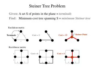
Euclidean metric Steiner Point Cost = 2 1 1 Cost = 3 Terminals 1 1 1 Rectilinear metric Cost = 6 Cost = 4 1 1 1 1 1 1 1 1 1 1 Steiner Tree Problem Given: A set S of points in the plane = terminals Find:Minimum-cost tree spanning S = minimum Steiner tree
Approximation Ratio = sup achieved cost optimal cost Steiner Tree Problem in Graphs Given: Weighted graph G=(V,E,cost) and terminals S V Find:Minimum-cost tree T within G spanning S Complexity: Max SNP-hard [Bern & Plassmann, 1989] even in complete graphs with edge costs 1 & 2 GeometricSTP NP-hard [Garey & Johnson, 1977] but has PTAS [Arora, 1996]
Approximation Ratios in Graphs 2-approximation [3 independent papers, 1979-81] Last decade of the second millennium: 11/6 = 1.84 [Zelikovsky] 16/9 = 1.78 [Berman & Ramayer] PTAS with the limit ratios: 1.73 [Borchers & Du] 1+ln2 = 1.69 [Zelikovsky] 5/3 = 1.67 [Promel & Steger] 1.64 [Karpinski & Zelikovsky] 1.59 [Hougardy & Promel] This paper: 1.55 = 1 + ln3 / 2 Cannot be approximated better than 1.004
Steiner points = P Terminals = S Steiner tree Approximation in Quasi-Bipartite Graphs Quasi-bipartite graphs =all Steiner points are pairwise disjoint Approximation ratios: 1.5 + [Rajagopalan & Vazirani, 1999] This paper: 1.5 for the Batched 1-Steiner Heuristic [Kahng & Robins, 1992] 1.28 for Loss-Contracting Heuristic, runtime O(S2P)
Steiner tree Approximation in Complete Graphs with Edge Costs 1 & 2 Approximation ratios: 1.333 Rayward-Smith Heuristic [Bern & Plassmann, 1989] 1.295 using Lovasz’ algorithm for parity matroid problem [Furer, Berman & Zelikovsky, TR 1997] This paper: 1.279 + PTAS of k-restricted Loss-Contracting Heuristics
Terminal-Spanning Trees Terminal-spanning tree = Steiner tree without Steiner points Minimum terminal-spanning tree = minimum spanning tree => efficient greedy algorithm in any metric space Theorem: MST-heuristic is a 2-approximation Proof: MST<Shortcut TourTour = 2 • OPTIMUM
T K Full Steiner Trees: Gain • Full Steiner Tree = all terminals are leaves • Any Steiner tree = union of full components (FC) • Gain of a full component K, gainT(K) = cost(T) - mst(T+K)
FC K Loss(K) C[K] FC K Full Steiner Trees: Loss • Loss of FC K = cost of connection Steiner points to terminals • Loss-contracted FC C[K] = K with contracted loss
k-Restricted Steiner Trees k-restricted Steiner tree = any FC has k terminals optk = Cost(optimal k-restricted Steiner tree) opt=Cost(optimal Steiner tree) Fact: optk (1+ 1/log2k) opt [Du et al, 1992] lossk = Loss(optimal k-restricted Steiner tree) Fact:loss (K) < 1/2 cost(K)
mst mst gain(K1) gain(K1) gain(K2) loss(K1) gain(K3) gain(K2) reduction of T cost reduction MST(H) gain(K4) loss(K2) gain(K3) loss(K4) loss(K3) loss(K3) gain(K4) loss(K2) loss(K4) loss(K1) opt opt Loss-Contracting Algorithm Input: weighted complete graph G terminal node set S integer k Output: k-restricted Steiner tree spanning S Algorithm: T = MST(S) H = MST(S) Repeat forever Find k-restricted FC K maximizing r = gainT(K) / loss(K) If r 0 then exit repeat H = H + K T = MST(T + C[K]) Output MST(H)
mst - optk Approx optk + lossk ln (1+ ) lossk Approximation Ratio Theorem: Loss-Contracting Algorithm output tree Proof idea: New Lower Bound Let H = Steiner tree and gain C[H] (K) 0 for any k-restricted FC K Then cost(C[H]) = cost(H) - loss(H) optk With every iteration, cost(T) decreases by gain(K)+loss(K) Until cost(T) finally drops below optk The total loss does not grow too fast Similar techniques used in [Ravi & Klein, 1993/1+ln 2-approximation]
mst - optk Approx optk + lossk ln (1+ ) lossk Quasi-bipartite and complete with edge costs 1 & 2 1.28 mst 2•(optk - lossk) - it is not true for all graphs :-( Approx optk + lossk ln ( - 1) partial derivative by lossk = 0 if x = lossk / (optk - lossk ) is root of 1 + ln x + x = 0 then upper bound is equal 1 + x = 1.279 optk lossk Derivation of Approximation Ratios General graphs 1+ ln3 /2 mst 2•opt partial derivative by lossk is always positive lossk 1/2 optk maximum is for lossk= 1/2 optk
Open Questions • Better upper bound (<1.55) • combine Hougardy-Promel approach with LCA • speed of improvement 3-4% per year • Better lower bound (>1.004) • really difficult … • thinnest gap = [1.279,1.004] • More time-efficient heuristics • Tradeoffs between runtime & solution quality • Special cases of Steiner problem • so far LCA is the first working better for all cases • Empirical benchmarking / comparisons