Download
1 / 38
390 likes | 530 Vues
Experiments on subaqueous mass transport with variable sand-clay rati o. Fabio De Blasio Trygve Ilstad Anders Elverhøi Dieter Issler Carl B. Harbitz International Centre for Geohazards Norwegian Geotechnical Institute, Norway Dep. of Geosciences, University of Oslo, Norway.

E N D
Experiments on subaqueous mass transport with variable sand-clay ratio Fabio De Blasio Trygve Ilstad Anders Elverhøi Dieter Issler Carl B. Harbitz International Centre for Geohazards Norwegian Geotechnical Institute, Norway Dep. of Geosciences, University of Oslo, Norway. . In cooperation withthe SAFL group, University of Minnesota
Basic problem! • How can we explain that 10 - 1000 km3 of sediments can • move100 - > 200 km • on < 1 degree slopes • at high velocities • ( -20 - > 60 km/h) • Debris • flow
Inferring the dynamics of subaqueous debris flow • Field observations (long runout, outrunner blocks, geometry of sandy bodies, velocity...) • Experiments: • (Experiments +Numerical modeling) × Extrapolation Field • composition change • Physical understanding and numerical simulation • Important application: • Emplacement of massive sand in deep water • Offshore geohazards
Experimental settingsSt. Anthony Falls Laboratory Experimental Flume: “Fish Tank” turbidity current debris flow 6° slope 10 m Video (regular and high speed) and pore- and total pressure measurements
How to explain the various styles of run out! Subaerial Short and thick Subaqueous Thin and long
High clay content – video record Turbidity current Hydroplaning debris flow
High speed video record (250 frames/sec) Flow behavior - High clay content( 30 % kaolinite)
Low clay content – video record Turbidity current Dense flow Deposition of sand
Debris flows- low clay content (5%) Turbulent front Deposition of sand
High clay content- • - Plug flow- “Bingham” • High sand content • Macro-viscous flow? • Divergent flow in the • shear layer
Pore pressure Total pressure Flow Pore pressure Flow Pressure Flow Time Pressure interpretation Grains in constant contact with bed Total pressure Pressure Fluidized flow Time Pressure Rigid block over a fluid layer Time
Pressure measurements at the base of a debris flow as pressure develops during the flow Low clay content High clay content Total pressure Hydrostatic pressure
Material from the base of the debris flow is eroded and incorporated into the lubricating layer. L2 Ls L1 H2 Hs H1 Downslope gravitational forces Bottom shear stresses
Detachment/stretching dynamics Neglected physics: • Changing tension due to slope and velocity changes • Friction, drag and inertial forces on neck • Changes in material parameters of neck due to • shear thinning, accumulated strain and wetting, crack formation • More sophisticated treatment is possible • Coupled nonlinear equations, use a numerical model • Main difficulty is quantitative treatment of crack formation and wetting and lubricating effects
Clay rich sediments • Visco-plastic materials • Model approach: • ”Classical Bingham fluid” (“BING”) • R-BING: Remolding of the sediment during the flow • H-BING: Hydroplaning/Lubricating
Shear layer Velocity profile of debris flows Bingham fluid • Classical Bingham fluid: • Yield strength: constant during flow • Bingham fluid – with remolding (R-BING): • The yield strength is allowed to vary during flow Plug layer Pluglayer
Water film/lubricating layer shear stress reduction in a Bingham fluid u=1 Lid(Debris flow) 1 1 =1 Water, w, w, uw =1- Mudm, m, um 1+ 1 u 1 1 1- 1- (R-)/ 1 u Plug layer Shear layer Velocity Shear stress 1+ R(1+)/
What happens during flow at low clay content? • 1) disintegration of the mass: the yield stress drops dramatically • 2) settling and sand stratification within few seconds dependent on the clay content Reference solid fraction solid fraction in the slurry
Existing models adapted to low clay debris flows: e.g.: NIS model • Mud with plug and shear layers • plasticity, viscosity, and visco-elasticity • dry friction (no cohesion in code) • dynamic shear (thinning) • dispersive pressure
Iverson- Dellinger model • Depth integrated, three-dimensional model • Accounts for the exchange of fluid between different parts of the slurry due to diffusion and advection. • Limitations for our purpose: water content of the slurry must not change, no cohesion, no turbulence
In short: high clay debris flows • Viscoplastic behaviour • Vertically quasi-homogeneous • Hydroplaning/lubrication • Dynamical forces important • The material remains compact • Front detachment/outrunner block • Modeling: rheological flow, • Modified “BING” • THEY ARE VERY MOBILE BECAUSE OF LUBRICATION
Granular + turbulent behaviour Settling and vertical layering (“Brazil Nut Effect” ) Lubrication only at the very beginning The material breaks up catastrophically Blocks do not form Modeling: Fluid dynamics + granular THEY ARE VERY MOBILE BECAUSE OF DRAMATIC DROP IN YIELD STRESS AND FLUIDISATION IN THE SAND LAYER In short: low clay debris flows
Conclusions • Slurries with a high clay content: • transported over long distances preserving the initial composition • Slurries with low clay content: • sandy materials may drop out during flow, alternatively being transformed into turbidity currents • Flow behavior: • Strongly influenced by the amount of clay versus sand in the initial slurry
Iverson-Dellinger model • the Coulomb frictional force (diminished of the water pressure at the base of the debris flow), • the fluid viscous shear stress, • the earth-pressure force (namely, the lateral forces generated in the debris flow due to differences in the lateral pressure), • the earth-pressure contribution of the bed pressure, • a diffusive term of water escaping from the bottom, • an earth-pressure term along the lateral (z) direction, • the diffusive term of water along the lateral direction, and finally • the pressure at the base of the debris flow.
Conclusions • At high clay content: • a thin water layer intrudes underneath the front part = lubrication! • progressive detachment of the head • the thin water underneath the head is a supply for water at the base of the flow • a shear wetted basal layer with decreased yield strength is formed • At low clay content: • water entrainment at the head of the mass flow • low slurry yield stress = particles settlement and continuous deposition • a wedge thickening depositional layer is developed some distance behind the head • viscous effects in the diluted flow, Coulomb frictional behavior within the dense flow. High pore pressures → near liquefaction.
Dispersive pressure • When solid particles are present • Particles forced apart • Ability to move large particles • proportional to square of the particle size for given shear rate (Bagnold, 1954) • larger particles forced towards area of least shear (up and front) • Further research required
shear stress dynamic viscosity yield strength shear rate Velocity profile of debris flows Bingham fluid Plug layer Shear layer Yield strength: constant during flow
u=1 Lid(Debris flow) 1 1 =1 Water, w, w, uw =1- Mudm, m, um 1+ 1 u 1 1 1- 1- (R-)/ 1 u Water film shear stress reduction in a Bingham fluid Plug layer Shear layer Velocity Shear stress 1+ R(1+)/
Debris flows- high clay content A: 32.5 wt% clay, hydroplaning front Dilute turbidity current B: 25 wt% clay hydroplaning front D: Behind the head, increasing concentration in overlying turbidity current
Debris flows- low clay content (5%) Turbulent front Deposition of sand