Download
1 / 12
120 likes | 228 Vues
9. Testing Model Linearity. Modified Beale’s Measure (p. 142-143) Total model nonlinearity (p. 144) Intrinsic model nonlinearity (p. 145) For total and intrinsic model nonlinearity measures, also see the UCODE_2005 documentation, table 38, p. 214. Testing for Linearity.

E N D
9. Testing Model Linearity Modified Beale’s Measure (p. 142-143) Total model nonlinearity (p. 144) Intrinsic model nonlinearity (p. 145) For total and intrinsic model nonlinearity measures, also see the UCODE_2005 documentation, table 38, p. 214.
Testing for Linearity • Linear confidence intervals are calculated under the assumption that the model is linear in the vicinity of the parameter estimates, where “vicinity” relates to the width of the interval. This, in turn, relates to the significance level of the interval. • If the model is not effectively linear, then the linear confidence intervals are not accurate, and need to be used as a rough approximation of the parameter uncertainty. • The modified Beale’s measure (Cooley and Naff, 1990) can be used to test whether a model is linear for parameter values close to the parameter estimates. To compute this measure: • Sets of parameter values close to the optimized parameter values are generated. • A forward model run is executed for each generated parameter set, to compute the simulated equivalents of the observations. • Linearized estimates of the simulated heads and flows are also calculated using the generated parameter sets. • The modified Beale’s measure is calculated.
Testing for Linearity • Parameter values are generated using the parameter variance-covariance matrix. 2NP’ parameter sets are generated. The two parameter sets corresponding to parameter j are: • If i=j, V(bj,bi) is the parameter variance, and if ij, V(bj,bi) is the covariance between parameters i and j. • F(NP’,ND+NPR-NP’) is the value from the F-distribution for NP’ and ND+NPR-NP’ degrees of freedom and significance level . For testing linearity of the model with respect to 95-percent confidence intervals, use = 0.05. • Generally, generated values of parameters with smaller variances will be closer to the estimated parameter values, and generated values of parameters with larger variances will be further from the estimated parameter values.
Testing for Linearity • The linearized estimates of the simulated values are calculated using the sensitivities of the simulated values to the model parameters, evaluated at the optimal parameter estimates:
Testing for Linearity • An example in which y is a function of only 1 parameter: Nonlinear model Linear model Linearized model
Testing for Linearity • Finally, the modified Beale’s measure is calculated as: • To check the degree of nonlinearity, the modified Beale’s measure is compared against critical values :
Testing for Linearity • After a successful optimization with UCODE_2005, do the following. • Log-transform any parameters for which solutions are invalid using possible values (for example, K’s in ground-water models). Adjust the prior information equations as needed. • Run UCODE_2005 with Optimize=yes • Run UCODE_2005 with Linearity=yes to compute the parameter sets and to compute the linearized simulated values • Run program Model_Linearity to calculate the modified Beale’s measure and the associated critical values • DO EXERCISE 7.3a (page 155): Calculate the modified Beale’s measure (for now just with the original weighting on the prior information)
Total and Intrinsic Model Nonlinearity • Total Model Nonlinearity • Performs much like the modified Beale’s measure. • Intrinsic Model Nonlinearity • Measures the nonlinearity that could not be diminished with any type of parameter transformation. • Some statistics, such as Cook’s D, are only affected by intrinsic model nonlinearity. • Application to ground-water models by Yager (1998, WRR)
Calculating the model nonlinearity measures • Run UCODE_2005 with Optimize=yes, starting from other than the optimized parameter values. • Run UCODE_2005 with Linearity=yes • Run Model_Linearity (no user-prepared files) Beale’s measure • Run Corfac_Plus (user-prepared file needed, but very simple; ex7.3_ucode.corfac) • Run UCODE_2005 with ModelLinearityAdv=Conf • Run Model_Linearity_ADV (no user-prepared files) • Repeat entire analysis using a more realistic statistic on the prior information.
ex7.3_ucode.corfac Begin Correction_Factor_Data Keywords ConfidenceOrPrediction=confidence RegressionUsedTrueCov=yes Read_Cov=no End Correction_Factor_Data Begin Parameter_List Table #This is needed for the combined model linearity measure nrow=6 ncol=1 columnlabels ParameterName HK_1 VK_CB HK_2 K_RB RCH_1 RCH_2 End Parameter_List
Total and Intrinsic Model Nonlinearity • Exercise 7.3b
From output file from Model_Linearity_ADV ########################################################## ########### ########### TOTAL NONLINEARITY (BNT).......... = 45.433 ########### INTRINSIC NONLINEARITY (BNI)...... = 0.12908 ########### ###########CRITICAL VALUES FOR BOTH MEASURES: ########### >1.0 highly nonlinear ########### 0.09 to 1.0 non-linear ########### 0.01 to 0.09 moderately nonlinear ########### <0.01 effectively linear ##########################################################