Download
1 / 38
590 likes | 1.12k Vues
Representation of Curves and Surfaces. Graphics Systems / Computer Graphics and Interfaces. Representation of Curves and Surfaces. Representation of surfaces : Allow describing objects through their cheeks. The three most common representations are: Polygonal mesh

E N D
Representation of Curves and Surfaces Graphics Systems /Computer Graphics and Interfaces COMPUTER GRAPHICS AND INTERFACES / GRAPHICS SYSTEMS JGB / AAS 2004
Representation of Curves and Surfaces Representation of surfaces: Allow describing objects through their cheeks. The three most common representations are: • Polygonal mesh • Bicúbicas parametric surfaces • Quadratic surfaces Parametric representation of curves: Important in computer graphics and 2D because of parametric surfaces are a generalization of these curves. "Tea-pot" modeled by smooth curved surfaces (bicúbicas). Reference model in computer graphics, especially for new techniques of realism texture and surface testing. Created by Martin Newell (1975) COMPUTER GRAPHICS AND INTERFACES / GRAPHICS SYSTEMS JGB / AAS 2004
Polygonal Mesh Polygonal Mesh: Is a collection of edges, vertices and polygons interconnected so that each edge is shared only a maximum of two polygons. 3D object represented by polygon mesh. Curve polyline Section of a curved object. The approximation error can be reduced by increasing the number of polygons. COMPUTER GRAPHICS AND INTERFACES / GRAPHICS SYSTEMS JGB / AAS 2004
Polygonal Mesh Characteristics of polygonal mesh: • An edge connects two vertices. • A polygon is defined by a closed sequence of edges. • An edge is shared by two adjacent polygons or 1. • A vertex is shared by at least two edges. • All edges are part of a polygon. The data structure for represent the polygonal mesh can have multiple configurations, which are evaluated by memory space and Processing time needed to get a response, for example: • Get all the edges that join a given vertex. • Determine the polygons that share an edge or a vertex. • Determine the vertices attached to an edge. • Determine the edges of a polygon. • Plot the mesh. • Identify errors in the representation, as the lack of an edge, vertex or polygon. COMPUTER GRAPHICS AND INTERFACES / GRAPHICS SYSTEMS JGB / AAS 2004
(X3, y3, z3) (X2, y2, z2) (X4, y4, z4) (X1, y1, z1) 4x 3x Polygonal Mesh . 1 Representation Explains: each polygon is represented as a list of coordinates of the vertices that constitute it. An edge is defined by two consecutive vertices and between the last and first on the list. P = ((x1, y1, z1), (x2, y2, z2), ..., (xn, yn, zn)) Evaluation of the data structure: • Memory consumption (repeated vertices). • There is an explicit representation of edges and vertices shared. • In the graphical representation of the same edge is "clipped"Drawn and more than once. • When you drag a vertex is necessary to know all the edges that share that vertex. COMPUTER GRAPHICS AND INTERFACES / GRAPHICS SYSTEMS JGB / AAS 2004
Polygonal Mesh . 2 Representation of Pointers to List of Vertices: each polygon is represented by a list of indices (or pointers) for a list of vertices. List of Vertices V = ((x1, y1, z1), (x2, y2, z2), ..., (xn, yn, zn)) V = (V1, V2, V3, V4) = (x1, y1, z1), (x2, y2, z2), ..., (x4, y4, z4)) P1 = (1,2,4) P2 = (4,2,3) Advantages: • Each vertex of the polygon mesh is stored only once in memory. • The coordinate of a vertex is easily changed. Disadvantages: • Hard to get the polygons that share a given edge. • The edges remain "clipped " and drawn once more. COMPUTER GRAPHICS AND INTERFACES / GRAPHICS SYSTEMS JGB / AAS 2004
Polygonal Mesh . 3 Representation of Pointers to List of Edges: each polygon is represented by a list of pointers to a list of edges, wherein each edge appears only once. In turn, each edge points to two vertices that define it and also stores the polygons which it belongs. A polygon is represented by P = (E1, E2, ..., En) and an edge as E = (V1, V2, P1, P2). If the edge belongs to only one polygon then P2 it is null. COMPUTER GRAPHICS AND INTERFACES / GRAPHICS SYSTEMS JGB / AAS 2004
Polygonal Mesh Advantages: • The graphic design is easily obtained by scrolling through the list of edges. Not repeating occurs clipping or drawing. • To fill (color) of the polygons works with a list of polygons. Easy operation is performed clipping on the polygons. Disadvantages: • Still not immediately determine the edges that focus on the same vertex. Solution Baumgart • Each vertex has a pointer to one of the edges (random) which focuses this vertex. • Each edge has pointers to the edges that cover a vertex. COMPUTER GRAPHICS AND INTERFACES / GRAPHICS SYSTEMS JGB / AAS 2004
Curves Cubic Motivation: Smooth curves represent the real world. • Representation by polygonal mesh is a first order approximation: • The curve is approximated by a sequence of linear segments. • Large amount of data (vertices) to obtain the curve precisely. • Unwieldy to change the shape of the curve, ie several points need to position accurately. • Are generally used polynomials grade 3(CurvesCubic), and the complete curve formed by a number of cubic curves. • degree <3 offer little flexibility in controlling the shape of the curves and for an interpolation between two points with the definition of the derivative at the end points. A polynomial of degree 2 is specified by three points that define the plane where the curve takes place. • degree> 3may introduce unwanted oscillations and requires more computational calculation. COMPUTER GRAPHICS AND INTERFACES / GRAPHICS SYSTEMS JGB / AAS 2004
Curves Cubic The representation of the curves is in the form PARAMETRIC: x = fx(T), y = fy(T) ex: x = 3t3 + T2 y = 2t3+ T The explicit form: y = f (x) and x: y = x3+2 X2 1. We can not have multiple values y for the same x 2. Curves can not describe with vertical tangents The implicit form: f (x, y) = 0 and x: x2+ Y2-R2= 0 1. Restrictions need to be able to model only part of the curve 2. Difficult join two curves smoothly COMPUTER GRAPHICS AND INTERFACES / GRAPHICS SYSTEMS JGB / AAS 2004
Curves Parametric cubic The figure shows a curve formed by two parametric cubic curves in 2D. COMPUTER GRAPHICS AND INTERFACES / GRAPHICS SYSTEMS JGB / AAS 2004
Curves Parametric cubic General representation of the curve: x (t) = axt3+ Bxt2+ Cxt + dx y (t) = ayt3+ Byt2+ Cyt + dy z (t) = azt3+ Bzt2+ Czt + dz0≤ t ≤ 1 Being: COMPUTER GRAPHICS AND INTERFACES / GRAPHICS SYSTEMS JGB / AAS 2004
Curves Parametric cubic The above representation is used to represent a single curve. Bring together the various segments of the curve? We intend joining a point geometric continuity and That have the same slope at the junction smoothness (continuity of the derivative). Ensuring continuity and smoothness at the junction is ensured by matching the derivatives (tangent) curves at the junction point. To this end calculates: With: COMPUTER GRAPHICS AND INTERFACES / GRAPHICS SYSTEMS JGB / AAS 2004
Curves Parametric cubic Types of Continuity: G0 - Zero geometric continuity curves join at a point. G1 - Geometric continuity is an the direction of the tangent vectors is equal. C1 - Parametric continuity 1 the tangent at the point of junction have the same direction and amplitude (the first derivative equal). Cn - Parametric continuity n curves have at the junction point all the same derivatives up to order n. COMPUTER GRAPHICS AND INTERFACES / GRAPHICS SYSTEMS JGB / AAS 2004
Curves Parametric cubic If we consider tas timeThe continuity C1 means that the speed of an object moving along the curve remains continuous The continuity C2 imply that the acceleration would also be continuous. At the junction point of the curve S the curves C0,C1 and C2 we have: Continuity G0 between SandC0 Continuity C1 between SandC1 Continuity C2 between SandC2 COMPUTER GRAPHICS AND INTERFACES / GRAPHICS SYSTEMS JGB / AAS 2004
Curves Parametric cubic Parametric continuity is more restrictive than the geometric continuity: For example: C1 implies G1 At the junction point P2 we have: Q2 and Q3 are G1 with Q1 Only Q2 C is1 with Q1 (TV1= TV2) COMPUTER GRAPHICS AND INTERFACES / GRAPHICS SYSTEMS JGB / AAS 2004
P4 R4 P1 R1 P3 P4 P2 P1 Curves Cubic Parametric - Types of Curves • Hermite curves • Continuity G1 at junction points • Geometric vectors: • 2 endpoints and • The tangent vectors at those points • Bezier curves • Continuity G1 at junction points • Geometric vectors: • 2 endpoints and • 2 points that control the tangent vectors such extremes • Curves Splines • Very extended family of curves • Greater control continuity at junction points (C Continuity1 and C2) COMPUTER GRAPHICS AND INTERFACES / GRAPHICS SYSTEMS JGB / AAS 2004
Common notation Matrix Geometric Matrix Base Matrix T Matrix Base:Characterizes the type of curve Matrix Geometric:A given geometrically conditions and contains curve related to the values of the curve geometry. COMPUTER GRAPHICS AND INTERFACES / GRAPHICS SYSTEMS JGB / AAS 2004
Common notation Conclusion 1: Q (t) is a weighted sum of the elements of the geometric vector Conclusion 2: Weights are cubic polynomials in t FUNCTIONS MIX (Blending functions) COMPUTER GRAPHICS AND INTERFACES / GRAPHICS SYSTEMS JGB / AAS 2004
Hermite curves Geometric vectors: COMPUTER GRAPHICS AND INTERFACES / GRAPHICS SYSTEMS JGB / AAS 2004
Hermite curvesMixing functions (Blending functions) Q (t) = (2t3-3t2+1) P1 + (-2t3+3 T2) P4 + (T3-2t2+ T) R1 + (T3-T2) R4 Mixing functions of Hermite curves, referenced by the element of the geometric vector that multiplies, respectively. COMPUTER GRAPHICS AND INTERFACES / GRAPHICS SYSTEMS JGB / AAS 2004
Hermite curves - Example Left: Functions of heavy mixture by the appropriate factor from the geometric vector. Center: Y (t) = sum of the four functions of the left Right: Hermite curve COMPUTER GRAPHICS AND INTERFACES / GRAPHICS SYSTEMS JGB / AAS 2004
Hermite curves - Examples - P1 and P4 fixed - R4 fixed - R1 varies in the direction - P1 and P4 fixed - R4 fixed - R1 varies in amplitude COMPUTER GRAPHICS AND INTERFACES / GRAPHICS SYSTEMS JGB / AAS 2004
Hermite curvesExample of Interactive Design • The extreme points can be repositioned • The tangent vectors can be changed by pulling the arrows • The tangent vectors are forced to be collinear (L continuity1) And R4 is displayed in the opposite direction (higher visibility) • It is common to have commands to force continuity G0, G1 or C1 Continuity at the junction: • K> 0 G1 • K = 1 C1 COMPUTER GRAPHICS AND INTERFACES / GRAPHICS SYSTEMS JGB / AAS 2004
Hermite curves COMPUTER GRAPHICS AND INTERFACES / GRAPHICS SYSTEMS JGB / AAS 2004
P3 P4 P2 P1 Bezier curves Vector Geometric: For a given curve demonstrates that compared with GH: R1 = Q '(0) = 3. (P2- P1) R4 = Q '(1) = 3. (P4- P3) GH M =HB . GB COMPUTER GRAPHICS AND INTERFACES / GRAPHICS SYSTEMS JGB / AAS 2004
Bezier curves • The same Bezier curve representation: Q (t) = t. MB . GB Q (t) = (1-t)3P1 + 3t (1-t)2P2 + 3t2(1-t) P3 + t3P4 COMPUTER GRAPHICS AND INTERFACES / GRAPHICS SYSTEMS JGB / AAS 2004
Bezier curves Additional information about the functions of Mixture: • For t = 0 Q (t) = P1 For t = 1 Q (t) = P4 The curve passes P1 and P4 • The sum at any point is 1. • It is noted that Q (t) is a weighted average of the four control points, Then the curve is contained within the polygon convex (2D) or convex polyhedron (3D) defined by these points, called the "convex hull". What advantage can we draw here? Q (t) = (1-t)3P1 + 3t (1-t)2 P2 + 3t2(1-t) P3 + t3P4 COMPUTER GRAPHICS AND INTERFACES / GRAPHICS SYSTEMS JGB / AAS 2004
Bezier curves Binding of Bezier curves Continuity G1: P4 - P3 K = (P5 - P4) With K> 0 i.e.P3P4 and P5 must be collinear Continuity C1: P4 - P3 K = (P5 - P4) Restricting K = 1 COMPUTER GRAPHICS AND INTERFACES / GRAPHICS SYSTEMS JGB / AAS 2004
Drawing of Cubic curves Two algorithms: 1. Evaluation x (t), y (t) and z (t) incremental values for t between 0 and 1. 2 Subdivision of the curve:. Casteljau Algorithm • Evaluation x (t), y (t) and z (t) Horner's rule reduces the number of multiplications, 11 additions and 10 to 9 and 10, respectively operations. f (t) = at3+ Bt2+ Ct + d = ((at + b). + T c). T + d • Casteljau algorithm Perform the recursive subdivision of the curve, stopping only when the curve in question is sufficiently "flat" to be able to be approximated by a line segment. Efficient Algorithm: 6 requires only shifts and 6 additions in each division. COMPUTER GRAPHICS AND INTERFACES / GRAPHICS SYSTEMS JGB / AAS 2004
Drawing of Cubic curves - Casteljau Algorithm Possible stopping criteria: - The curve in question is sufficiently "flat" to be able to be approximated by a line segment. - The four control points are on the same pixel. L2 = (P1+ P2) / 2, H = (P2+ P3) / 2, L3 = (L2+ M) / 2, R3 = (P3+ P4) / 2 R2 = (H + R3) / 2, L4 = R1 = (L3 + R2) / 2 COMPUTER GRAPHICS AND INTERFACES / GRAPHICS SYSTEMS JGB / AAS 2004
Drawing of Cubic curves Algorithm Calteljau void DrawCurveRecSub (curve,ε) {if (Straight (curve,ε)) DrawLine (curve); else { SubdivideCurve (curve,leftCurve, rightCurve); DrawCurveRecSub (leftCurve, ε); DrawCurveRecSub (rightCurve, ε); } } COMPUTER GRAPHICS AND INTERFACES / GRAPHICS SYSTEMS JGB / AAS 2004
Exercise COMPUTER GRAPHICS AND INTERFACES / GRAPHICS SYSTEMS JGB / AAS 2004
Cubic Surfaces Cubic surfaces are a generalization of cubic curves. The equation of the surface is obtained from the equation of the curve: Q (t) = T. M. G, being G constant. Switch to variable s:Q (s) = S. M. G By varying the points of the vector G3D eométrico along a path parameterized by t are obtained: The geometrical matrix is composed of 16 points. COMPUTER GRAPHICS AND INTERFACES / GRAPHICS SYSTEMS JGB / AAS 2004
Surface Hermite For the x coordinate: It is concluded that: COMPUTER GRAPHICS AND INTERFACES / GRAPHICS SYSTEMS JGB / AAS 2004
Surface Hermite COMPUTER GRAPHICS AND INTERFACES / GRAPHICS SYSTEMS JGB / AAS 2004
Bezier Surface The equations for the Bezier surface can be obtained in the same way that the Hermite, resulting in: The geometric matrix has 16 control points. COMPUTER GRAPHICS AND INTERFACES / GRAPHICS SYSTEMS JGB / AAS 2004
Bezier Surface Continuity C0 and G0is obtained by matching the four points of border control: P14P24P34P44 For G1 should be collinear: P13P14 and P15 P23P24 and P25 P33P34 and P35 P43P44 and P45 and (P14-P13) / (P15 - P14) = K (P24-P23) / (P25 - P24) = K (P34-P33) / (P35 - P34) = K (P44-P43) / (P45 - P44) = K COMPUTER GRAPHICS AND INTERFACES / GRAPHICS SYSTEMS JGB / AAS 2004