Download
1 / 59
590 likes | 689 Vues
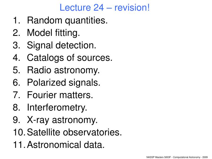
Lecture 24 – revision!. Random quantities. Model fitting. Signal detection. Catalogs of sources. Radio astronomy. Polarized signals. Fourier matters. Interferometry. X-ray astronomy. Satellite observatories. Astronomical data. 1. Random quantities.

E N D
Lecture 24 – revision! • Random quantities. • Model fitting. • Signal detection. • Catalogs of sources. • Radio astronomy. • Polarized signals. • Fourier matters. • Interferometry. • X-ray astronomy. • Satellite observatories. • Astronomical data.
1. Random quantities • Important properties of a random value Y: • The probability density p(y). • The mean or average • The variance • It is important to distinguish between the ideal values of these and estimates of them which one can calculate from a sample [y1,y2,...yN] of Y. • Although the ideal values are formally unattainable, in practice good estimates of them may be available. Eg: • There may be formulae which predict p, μ and (often most importantly) σ2(see eg radio astronomy). • Long-term calibration measurements can provide good estimates (true for most scientific instruments). These are not guar- anteed to exist!
1. Random quantities • Also often of interest is an integral over the probability density. p(y) y y0
1. Random quantities • Estimating the three properties from N samples of Y: • A frequency histogram serves as an estimate of p(y). • Estimate of the mean: • Estimate of the variance*: • The result of every (non-trivial) transformation of a set of random numbers is itself a random number. (For example, the estimators for the mean and variance.) Note: the ‘hats’ here mean ‘estimate’. *This formula was incorrect on slide 5 of lecture 3.
1. Random quantities • Measurements of some physical quantity: • We have a set of N measurements yi which are usually made at different values of some other essentially non-random quantities ri (eg at different times, positions, frequencies, etc etc) • It is often convenient to treat each measurement yi as a sum of signalsi, backgroundbi and noiseni. • The division between signal and background is made largely on grounds of convenience, or interest – it is a bit like the distinction between ‘useful’ plants and weeds.
1. Random quantities • The estimate μ^ will not approach the ideal μ of the noise at large N unless s+b=0. • The estimate σ^2 of the noise will not approach the ideal σ2 at large N unless s+b is constant. • Uncertainty propagation: if some random variable z is a function f(y) of other random variables y=[y1,y2,...yN], then
1. Random quantities • Often (not always!) the different yi are uncorrelated – ie, the value of one does not depend on another. In this case σi,j2=0 for i≠j and so • Examples (all uncorrelated):
2. Model fitting • Just as we do not have access to μ or σ2, neither do we have access to the ‘ideal’ quantities s(r) or b(r). • Model fitting is the process of estimating these quantities. • The usual practice is to propose a model which depends on a small number M of parameters Θ=[θ1,θ2,.. θM]. • The background can usually be much better estimated than the signal, because background tends to occur at similar levels in all data points, whereas signal is localized. • Hence it is often assumed that b^=b.
2. Model fitting • Steps in the estimation of s: • Decide on a model. • Choose a fitting statistic U: ie some formula which has the following properties: • It returns a single number. • It is a function of the data values yi and the model m(x). • U should be a smooth function of the parameters Θ, with a quadratic (=analytic) minimum. • The parameter values at that minimum should be, in some reasonable sense of the words, the best fit parameters, ie provide the ‘best’ estimate of the ideal, unattainable s. • Calculate uncertainties, and the model plausibility.
2. Model fitting • Types of U: first I’ll look at the method of least squares. • This prescribes a formula for U which is essentially a ratio between variances. The estimate σ^2 we make from our data goes on the numerator, whereas the denominator is the predicted σ2. • Before writing this down, let us reconsider the formula for σ^2. Adapting the formula on slide 4 gives: • However, in general, this gives too small a value. And the larger the number M of parameters, the greater this error. This is because, as M is increased, the model can better and better follow the ups and downs of the noisy part of y.
2. Model fitting • A more accurate value is given by • The difference between the number N of data points and the number M of parameters to be fitted is called the number of degrees of freedom. • Note that the standard formula for σ^2 has N-1 degrees of freedom because μ^ represents a fitted model with 1 parameter. • Now at last we can construct our ratio. This U formula is • Another name for this is reduced chi squared or χ2red.
2. Model fitting • χ2 itself is the same formula, but without dividing by the degrees of freedom: • It is a funny notation, because no-one seems to think or care what χ might be. • Now we want to consider two related questions about this choice of U: • Can we tell from the best-fit value of U how good our choice of model was? • We have best-fit values of the parameters – can we also get their uncertainties?
2. Model fitting • The model is our hypothesis. It represents what we think the signal s(r) is doing. • There is an infinite choice of models. We cannot prove any given model is correct, only disprove it. • But how do we do this? • If the model choice is good, then the estimate σ^2 ought to be close to σ2; in other words, the value of χ2red in this case ought to be close to 1. • But suppose χ2red=1.04, or 2, or 7641. How ‘close’ to 1 is still good?
2. Model fitting • Whatever U formula we chose, we cannot decide whether the model is good or not without knowing the probability distribution of U. • Remember that U, as a function of random variables, is therefore itself a random variable, therefore has a p(U). • To test our model hypothesis, after we have done the fitting, and obtained Ubest fit, we have to: • Obtain p(U). • Calculate the probability If P is small, our model is suspect; in doubt; probably no good; has failed the test.
2. Model fitting • Sometimes, for certain choices of U, this distribution is a known function. U=χ2red is an example of this happy situation: in this case p(U) is an easily calculable function, and more importantly, so is P(U≥Ubest fit): where Q is the complementary incomplete gamma function.
2. Model fitting • For Poisson data, if we replace σi2 in the formula by mi,best fit, the probability distribution is unchanged (still χ2). • Thus we can easily use this formula for U to assess the worth of the model. • We can not use it to obtain mbest fit in the first place though, because the result is known to be biased. • An unbiased fitting formula has been devised by K Mighell: But the probability distribution for this is not known.
2. Model fitting • Uncertainties in the parameters: • If, for U= χ2red, we calculate the matrix H of second derivatives of U vs the model parameters, then the cross-correlation σij2 between parameters i and j (aka the square in the uncertainty if i=j) is the i,jth element of H-1. • Another form of U is the likelihood: • Suppose we know the probability distribution p(y) of y. Eg or
2. Model fitting • If, for every data point yi, we replace <y> in these expressions by our model m(Θ), then multiply all the probabilities together for i in [1,N], we have an expression for the likelihood L of a given set of parameters Θ. The best fit parameter values are taken to be those which maximize L. • Two further modifications are usually made: • Since the numbers are often very small, it is more convenient to work with log(L); • A minimization algorithm will need to work with the negative of the likelihood, ie the expression to minimize is –log(L).
3. Signal detection. • This is like model fitting, but we start with a special class of model: one which contains only background. • Often we don’t need to do the fitting part, because we have obtained a good estimate of the background from other sets of data. • All we have to do is test the model. • Remember that a model is our hypothesis about what lies behind the data. • This signal-less model is called the null hypothesis (‘null’ is from the Latin for ‘nothing’).
3. Signal detection. • The model testing proceeds exactly the same as before: • Calculate U for the null hypothesis model. • eg for U=χ2 this would be • Calculate the probability P(U≥Unull). • If this value is small, then the null hypothesis fails the test. Deduction: there probably is some signal present.
3. Signal detection • This is ok, but it may not be the most sensitive way to detect signals. This is because signal and background usually have different spatial scales: • Background usually extends over many data points; • Signal usually extends only over a few data points. • Thus, if one uses the whole data set to calculate U, a small signal may be swamped among the background and noise. • Some selection and filtering are usually done before applying the test.
3. Signal detection • A likelihood ratio between the likelihood Lbest calculated for best fit of a normal model m=b+s(Θ), and the likelihood Lnull for m=b alone, can also be used to test the null hypothesis. • W Cash has shown that for where M is the number of fitted parameters. • Don’t get confused though – this is a test of the null hypothesis, not of the best fit - a low value of this P means the null hypothesis is probably wrong and therefore there is some signal there.
3. Signal detection • Significance: • If you only have 1 random value y, and you want to decide whether it contains ‘signal’ or just ‘background’. • Eg the assignment question in which you had some values of the Stokes parameter V, plus its uncertainty. In this case the ‘background’ was zero. The question was, is there some ‘signal’ (ie a non-zero value of V) present. • The way to do this is to compare y-b with the uncertainty σy(this σ is the ‘expected’ standard deviation, calculated from sources other than the single data point). • The ratio (y-b)/σy is called the significance. • If the ratio is about 1, then you might say “y is consistent with the background value.” Ie you can’t rule out the null hypothesis. • Sometimes for a ratio X, you will hear people call this a “X-sigma detection.” X=5 is a commonly used yardstick for a detection which is judged to be significant.
4. Catalogs of sources. • Source detection is a special case, in which the model to be fitted is • The difficulty is that one usually doesn’t know the value of M. • So one has to assume that the sources are not confused – in other words that the separation between sources is usually greater than the size or extent of each si. Then one can use for m.
4. Catalogs of sources. • The value of amplitude A at which the source is detected about ½ the time is the sensitivity. • Different detection methods give differing sensitivities. • The completeness is the estimated fraction of sources above a certain A which are detected. • Eg “the survey is 90% complete above a flux of 10-13 erg cm-2 s-1.” • Suppose: • We test the null hypothesis at N locations. • We decide to label as sources all locations where Unull≥α. Then our catalog of sources will contain Nα false positives – ie places at which Unull≥α but where in reality there is no source. • (But! We can’t know which are real and which are false.) The fraction of false positives is a measure of the reliability of our survey.
4. Catalogs of sources. • Of interest is the frequency distribution of source amplitudes, n(A). • Often one talks of the source flux or flux density rather than amplitude: • Examples of units are erg cm-2 s-1 for x-ray and janskys for radio; • The symbol used is often S. • Hence n(S) is more common notation. • If the sources are distributed uniformly in space (known as a Euclidean distribution), n(S) will be a power law, with index=-2.5; in other words,
4. Catalogs of sources. • n(S) is estimated in the usual way: via a histogram. • Perhaps more often one makes a reverse cumulative histogram, to show the total number N(>S) of sources of flux ≥ S. • If n is a power law, so is with an index greater by 1. So in the Euclidean case, the index of N is -1.5.
5. Radio astronomy. • Radio dishes are reflectors just the same as mirrors of optical telescopes. Just the terminology is sometimes a bit different. • Instead of PSF one refers to the beam. • They are sensitive to radiation from a small area in the sky, of angle ~ λ/D. • The beam nearly always has sidelobes though. • Unlike optical detectors, radio detectors are polarized – the output voltage varies between a maximum and zero, depending on the polarization state of the incoming radiation. • Sometimes the detector is most sensitive to linear polarized radiation at a given angle, sometimes to left- or right-circularly polarized radiation. • Often these days, two detectors of opposite polarization are placed at the focus.
5. Radio astronomy. • Radio signals are nearly always noise-like. As such they can be mimicked by: • placing a resistor at a certain temperature across the input terminals to the detection electronics. or • pointing the antenna directly at a surface with the same temperature as the above resistor! • Because the noise power spectral density from such a resistor is equal to kT watts Hz-1 (kT is Boltzmann’s constant times the temperature in kelvin), radio engineers are in the practice of expressing all noise powers in terms of temperatures.
5. Radio astronomy. • Since powers are additive, so are the associated temperatures. • Thus the total output noise temperature can be expressed as a sum of several terms: • Such temperatures are most of the time not ‘real’ in the sense that they are numbers you could read off a thermometer somewhere. They are just a handy way of expressing power spectral density. • For example, the ‘real’ temperature of the ground is about 300K, but Tbackground in the above sum won’t be 300K unless the antenna is pointed right at the ground. Normally you will only get a little contribution from this hot surface from reflections and from far sidelobes. Ttotal = Tsource + Tbackground + Tatmosphere + Tsystem
5. Radio astronomy. • The uncertainty of a noise temperature is • For a point source of flux density S W m-2 Hz-1, the power spectral density where α varies from 0 to 1 depending on the relative polarization of radiation and detector, • (α=0.5 if the radiation is unpolarized) and Ae is the effective area of the antenna in m2.
5. Radio astronomy. • From these and from we have and This last is roughly equal to the limiting sensitivity of the telescope – ie the minimum flux point source which can be detected. (Technically you’d want to set the detection threshhold at 5σ or so.) In W m-2 Hz-1. You have to multiply by 1026 to convert to janskys. In W m-2 Hz-1. You have to multiply by 1026 to convert to janskys.
6. Polarized signals. Stokes parametersI, Q, U and V. I = total intensity. Q = intensity of horizontal pol. U = intensity of pol. at 45° V = intensity of left circular pol. V axis U axis Therefore need 4 measurements to completely define the radiation. Q axis Polarization angle is Polarization fraction d: Visualize with the “Poincaré sphere.” of radius I.
6. Polarized signals. • Depolarization: basically due to mixing of many slightly different, uncorrelated source polarizations within the width of the beam. • Faraday rotation of the polarization angle: where D is the distance from the source, Ne is the average number density of electrons along that path, and B is the average magnetic field. • Enhances depolarization because uneven DNeB within the beam amplifies differences between polarization angles. radians
7. Fourier matters. • What is the difference between • A Fourier series (FS); • A Fourier transform (FT); • A discrete* Fourier transform (DFT); • The Fast Fourier Transform (FFT)? • A Fourier series starts with a function f(t) defined on an interval [0,T]. Its FS to order N-1 is where *‘Discrete’ and ‘discreet’ mean different things – consult a dictionary!
7. Fourier matters. • The FT of f(t) (sometimes indicated F{f}) is: FTs are known for some functions, but not for others. They can’t in general be calculated exactly. • The DFT is the nearest one can get to a FT which is calculable. If f(t) is sampled at N evenly-spaced points within the interval [0,T], then the DFT is defined as
7. Fourier matters. • The relation of f’ to f is the same as F’ to F: In other words, f’ is f wrapped or aliased in a cyclic fashion at the interval boundaries 0 and T. • The FFT is not some new formula, it is a fast computer algorithm for calculating the DFT.
7. Fourier matters. • The convolution integral is • Its FT is: • The correlation integral between two functions f and g is closely related: • Its FT is: The * here denotes complex conjugation.
7. Fourier matters. • From that it is pretty clear that an autocorrelation (correlation of a function against itself) must be real-valued. • The FT of an autocorrelation of f is called the power spectrum of f. • The normalized, zero-lag correlation is just the average of the product of f and g:
8. Interferometry. Coordinate system: w u dθ l Phase centre m into the page. (1-l2)1/2 v into the page. θ u1,2 (u component of the baseline vector b1,2.) 2 1 w1,2 2
8. Interferometry. • The zero-lag complex correlation <y1y2> between the signals from the two antennas gives the spatial coherence function of the radiation • where • Multiplying by exp(2πiw) gives the visibility function: • The approximation is good provided πw(l2+m2)<<1.
8. Interferometry. • The really important points are: • The visibility function V is the inverse FT of the (slightly modified) sky intensity I’. • The multiplication of <y1y2> by exp(2πiw) is in reality accomplished by delaying the signal from each jth antenna by tlag=wjλ/c. • Baselines are separations between the antennas, measured in wavelengths, and projected onto the reference plane. • The phase centre is the direction normal to the reference plane.
8. Interferometry. A baseline separation Phase centre Reference plane Correlator delay delay delay Signals are selectively delayed so that plane waves from the phase centre arrive at the correlator in phase.
8. Interferometry. • The real-life process of interferometry: Cross-correlation effects an inverse FT. The visibility function V. The sky brightness distribution I. CLEAN or other deconvolution. Sampling Gridding, discrete FT. The dirty image D=I*B. VxS Gridding, discrete FT. The dirty beam B. The sampling function S
9. X-ray astronomy. • Imaging: • Wolter optics: • Grazing incidence, otherwise x-rays won’t reflect. • A paraboloid mirror followed by hyperboloid. • The effective area of a Wolter mirror shows a pronounced fall-off as the angle of incidence departs from the optic axis. Called vignetting. • The Wolter PSF also changes significantly across the field of view. • A ‘Coded Mask’ is another way to ‘image’ x-rays, and the only way to image gamma rays. • Actually it more resembles interferometry – the image is obtained by a Fourier technique.
9. X-ray astronomy. • Detection: • State-of-the-art detectors are CCDs. • An optical-wavelength the CCD accumulates charge from many low-energy photons. • At x-ray wavelengths, all the charge comes from just 1 high-energy photon. • This allows the energy of the photon to be measured. • Patterns of charge in adjacent pixels have to be interpreted by software ‘x-ray events’. • Thus the whole data processing is event-based rather than brightness-based; flux measurement is based on integers rather than floating-points. • Hence it is dominated by Poisson statistics.
9. X-ray astronomy. • Frames: • Longish time accumulating photons; • Too bright a source more than 1 photon per pixel per frame, called pileup. • Shortish time reading the data out. • Serial readout – slow – OOTEs – ‘dead time’. • Hardness ratios are a crude measure of an x-ray spectrum. • With a ‘proper’ spectrum, if it is a power law, you have to be careful whether you are talking about number of photons per unit photon energy, or total energy per unit photon energy. The respective spectral indices differ by 1.
10. Satellite observatories. • You need to know the orientation of the satellite in space. • (Remember too that this usually varies with time.) • For this, we define: • a sky coordinate frame with the x axis at RA=0, dec=0, the y axis at RA=6 hr, dec=0 and a a z axis at dec=90; • a spacecraft coordinate frame comprising three orthogonal vectors ax, ay and az; • an attitude matrix such that ax occupies row 1, ay row 2 and az row 3 (all vectors expressed in Cartesian coordinates of the sky frame).
10. Satellite observatories. • For example, if the spacecraft is pointing at RA=3 hr, dec=+30, and if it has 90 degrees of roll, the corresponding attitude matrix is: If you try to check this, but get figures which don’t agree, keep in mind the possibility (even likelihood) that I made an error!
10. Satellite observatories. • The instruments on the spacecraft are in general, not precisely aligned with the s/c coordinate axes. • Thus they need their own coordinate systems. • The difference between the two is called the boresight matrix for that instrument. • The 3 vectors bx, by and bz which define the instrument’s Cartesian coordinate system are expressed in the basis of the spacecraft coordinate system. • bx forms row 1, etc of the boresight matrix.