Download
1 / 25
371 likes | 757 Vues
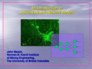
An Introduction to Artificial Neural Network Models. John Meech, Norman B. Keevil Institute of Mining Engineering, The University of British Columbia. What are Artificial Neural Networks ?. Artificial Neural Networks: A class of models that mimic the functioning of the human brain.

E N D
An Introduction to Artificial Neural Network Models John Meech, Norman B. Keevil Institute of Mining Engineering, The University of British Columbia
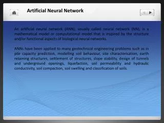
What are Artificial Neural Networks ? Artificial Neural Networks: A class of models that mimic the functioning of the human brain There are several classes of ANN models. They differ from one another depending on • The problem type Prediction, Classification, Clustering • The structure of the model • The algorithm used to reduce error Our focus here is on: Feed-forward Back-propagation Neural Networks which are used for Prediction and Classification problems.
Technology mirrors Biology – Intelligent Information Processing Dendrites Cell Body Axon Synapse Most important processing unit in the human brain: a class of cells called –NEURONS Hippocampal Neurons Source: heart.cbl.utoronto.ca/ ~berj/projects.html Schematic • Dendrites– Receive information • Cell Body– Processes information • Axon– Carries processed information to other neurons • Synapse– Junction between Axon end and Dendrites of other Neurons
An Artificial Neuron Dendrites Cell Body Axon I1 Direction of flow of Information w1 w2 I2 O = f(S) f S . . . S = w1I1 +w2I2 +w3I3 +…+ wnIn wn In • Neuron receives inputs I1 I2 …Infrom other neurons or the environment • Inputs are fed-in through connections with "weights" (-∞ to +∞) • Total Input (S) = weighted sum of inputs from all sources • Transfer function (Activation function) converts the input to an output (O) • Output is sent to other neurons or to the environment
1 1 0.5 0 -1 (ex–e-x) _______ (ex + e-x) f(x) = Transfer Functions There are various choices for Transfer / Activation functions 1 0 Sigmoid Threshold 0 if x< 0 f(x) = 1 if x >= 1 Tanh 1 _______ (1 + e-x) f(x) = They are virtually the same function – simply scaled differently
(ex–e-x) (ex+e-x) _________ 2(ex + e-x) _________ 2(ex + e-x) + = (2ex) _________ 2(ex + e-x) = 1 1 _______ (1 + e-∞x) _______ (1 + e-2x) f(x)= f(x)= 0 if x< 0 f(x) = 1 if x >= 1 (ex–e-x) _______ (ex + e-x) f(x) = Transfer Functions – sa fait rien! Let's take the Tanh function: and ADD 1 and DIVIDE by 2: Voila! The Sigmoid function of the square of the summation! Now take the Sigmoid function and scale the summation to +∞: Et voila encore! The Threshold function! So they are all the same functions – simply scaled differently Transfer functions serve to scale the output between 0 and 1 or between -1 and +1
I1 I2 I3 I4 Direction of information flow O1 O2 ANN – Feed-forward Network A set of neurons form a ‘Layer’ Input Layer - Each neuron receives ONLY one input, directly from outside Hidden Layer - Connects Input and Output layers Output Layer - Output of each neuron directly goes to outside
ANN – Feed-forward Network The number of hidden layers is a design parameter – it can be: None One More Perceptron Network
I1 I2 I3 I4 O1 O2 ANN – Feed-forward Network • Within a layer, neurons are NOT connected to each other. • Neurons in one layer are connected to neurons ONLY in the NEXT layer. (Feed-forward) • Jumping of layer is NOT permitted All of these constraints (or rules) may be broken (and frequently are) by many ANN tools on the market
One particular ANN Model What is meant by a "particular" model ? Input: I1 , I2 , I3 Output: O Model: O = f(I1 , I2 , I3) The algebraic form of f( ) is too-complex to write down. • However, the model is characterized by • The number ofInput Neurons • The number of Hidden Layers • The number of Neurons in each Hidden Layer • The number of Output Neurons • The WEIGHTS of all the connections • The presence (or not) of a Bias node "Fitting" an ANN model involves specifying values for all these parameters among several other parameters
I2 I3 I1 -0.2 0.6 -0.1 0.1 0.7 0.5 0.1 -0.2 O Decided by the problem structure # Input Neurons = # of I’s # Output Neurons = # of O’s Free parameters An Example Input:I1, I2 , I3 Output:O Model:O = f(I1 , I2 , I3) Parameters Example # Input Neurons3 # Hidden Layers1 # Hidden Layer Neurons2 # Output Neurons1 Weights are Specified
I1 =1 I2=0.3 I3 =0.6 -0.73 = 0.5*1 – 0.1*(0.3) – 2.0*0.6 f(S) = 1 / (1 + e-S) f(-0.73) = 1 / (1 + e0.73) = 0.55 1.05 -0.73 Predicted Op = 0.112 f (1.05) = 0.256 f (-0.73) = 0.324 0.324 0.256 -2.068 f (-2.068) = 0.112 0.112 An Example Input:I1, I2 , I3 Output:O Model:O = f(I1 , I2 , I3) -2.0 0.6 -0.1 0.1 0.7 0.5 0.1 -0.2 Suppose Actual O = 0.9 Then Prediction Error = (0.9 - 0.112) =0.788
# Hidden Layers = ??? Try1 # Neurons in Hidden Layer = ???Try2 No fixed strategy. Use trial and error. Building an ANN Model Input:I1 ,I2,I3 Output:O Model:O = f(I1 , I2 , I3) # Input Neurons = # Inputs =3# Output Neurons = # Outputs =1 Architecture is now defined … Now to get the weights Given the Architecture, there are 8 weights to decide: W = (W1, W2, …, W8) Training Data: (Oi , I1i, I2i, …, Ini) i= 1,2,…,k Given a particular choice ofW, ANN predicts a value forO: (Op1,Op2,…,Opk) These are afunctionof W. Choose Wsuch that overall prediction errorEis minimized. E = (Oi – Opi)2
Back Propagation Feed forward Training the Model • Start with a random set of weights. • Feed the first observation set through the network • I1, I2,I3NetworkOp1;Error = (O1 – Op1) • Adjust the weights so that this error is reduced (so network fits the first observation) • Feed forward the second observation. Adjust weights to fit the second observation • Repeat until the last observation set is reached • This finishes oneCYCLEthrough the data • Perform many such training cycles till the overall prediction errorEis small. E = (Oi – Opi)2
Back Propagation Back Propagation • Each weight "shares the blame" for the prediction error with all of the other weights. • The Back Propagation algorithm decides how to distribute the blame among all weights and adjusts the weights accordingly. • A small portion of blame leads to small adjustment. • A large portion of blame leads to large adjustment. E = (Oi – Opi)2
Weight Adjustment by Back Propagation Opi is the prediction for theithobservation It is a function of the network weights vectorW= ( W1 , W2,….) Hence,E, the total prediction error is also a function ofW E( W) = [ Oi – Opi( W )] 2 Gradient Descent Method : For each individual weightWi , the update formula is: Wnew = Wold + * (E / S)Wold = Learning Parameter (0 to 1) An alternate variation is often used W(t+1) = W(t) + * (E / S)W(t) + * [W(t) - W(t-1)] = Momentum Parameter (0 to 1)
w1 w2 Geometric Interpretation of Weight Adjustment Consider a simple network with 2 inputs and 1 output and no hidden layer. There are only two weights whose values are needed. E( w1, w2) = [ Oi – Opi(w1, w2 ) ] 2 • Each pair of weights ( w1, w2 ) is a point on a 2-D plane. • For any such point we can get a value of E. • PlotEvs ( w1, w2 )to get a 3-D surface -Error Surface • Goal is to identify the pair for whichEis minimum • Identify pair for which height of error surface is minimum. • Gradient Descent Algorithm • Start with a random point( w1, w2 ) • Move to a "better" point( w'1, w'2 )where the height of error surface is lower. • Keep moving till you reach( w*1, w*2 ), where the error is minimum.
Back-Propagation Error-Summation Slope E = O – Op = O - f (S) = (1 + e-S)-1 E/S = -f’(S) = - · -e-S · -1(1 + e-S)-2 E/S = - e-S(1 + e-S)-2 but Op = (1 + e-S)-1 and 1 – Op = 1 - (1 + e-S)-1 = e-S (1 + e-S)-1 so Op · (1 – Op) = e-S (1 + e-S)-2 f’(S) = Op · (1 – Op)
Error Surface Local Minima Global Minima w* w0 Weight Space Searching the Error Surface
Dountil Convergencecriterion is met For i = 1 to # Training Data points Next i End Do Training Algorithm Decide on theNetwork Architecture (# Hidden layers, #Neurons in each Hidden Layer) Decide on theLearning and Momentum Parameters Initializethe Network with random weights Feed forwardthe ith observation to the Network Compute the prediction error on ith observation Back propagatethe error and adjust weights Check for Convergence E = (Oi – Opi)2
Convergence Criterion When should Training stop ? Ideally – when we reach theglobal minimaof the error surface How do we know when we have reached it ? We don’t … • Suggestion: • Stop if the decrease in total prediction error (since last cycle) issmall. • Stop if the overall changes in the weights (since last cycle) aresmall. Drawback: Error keeps on decreasing. We get avery good fit to training data. BUT …The obtained network haspoor generalizing poweronunseen data The phenomenon is known asOver-fittingof the Training data The network is said to haveMemorizedthe training data. - so that when anIin a training set is given,the network faithfully produces the correspondingO. - However forIvalues which the network has never seen, it predicts poorly.
Validation Error Training Cycle Convergence Criterion Alternate Suggestion: Partition the training data into aTraining setand aValidation set UseTraining set to build the model Validation set to test the performance of the model on unseen data Typically as we have more and more training cycles Error of Training set keeps on decreasing. Error of Validation set first decreases and then increases. Stop training when the error of Validation set starts increasing
Training Parameters Learning and Momentum Parameters - supplied by User: value lies between 0 and 1 What is the optimal values of these parameters? - No clear consensus on any particular strategy. - However, effects of wrong specification are well-studied. Learning Parameter Too big – Large leaps in weight space – risk of missing global minima. Too small – Takes long time to converge to global minima – Once stuck in local minima, difficult to get out of it. Suggestion Trial and Error – Try various choices of Learning and Momentum Parameters – See which choice leads to minimum prediction error
Summary • Artificial Neural Networks (ANN) – A class of models inspired by biological Neurons • Used for various modeling problems – Prediction, Classification, Clustering, .. • One particular subclass of ANN – Feed-Forward Back Propagation Networks • Organized in layers – Input, Hidden, Output • Each layer is a set of a number of Artificial Neurons • Neurons in one layer are connected only to Neurons in next layer • Each connection has a weight • Fitting an ANN model involves finding the values of these weights. • Given a training data set – weights are found by the Feed-Forward Back Propagation algorithm, a form of the Gradient Descent Method. • Network architecture as well as training parameters are decided by trial and error. Try different values and use the ones that give lowest prediction error.