Download
1 / 36
360 likes | 366 Vues
Computing Nash Equilibrium. Presenter: Yishay Mansour. Outline. Problem Definition Notation Last week: Zero-Sum game This week: Zero Sum: Online algorithm General Sum Games Multiple players – approximate Nash 2 players – exact Nash. Model. Multiple players N={1, ... , n}

E N D
Computing Nash Equilibrium Presenter: Yishay Mansour
Outline • Problem Definition • Notation • Last week: Zero-Sum game • This week: • Zero Sum: Online algorithm • General Sum Games • Multiple players – approximate Nash • 2 players – exact Nash
Model • Multiple players N={1, ... , n} • Strategy set • Player i has m actions Si = {si1, ... , sim} • Siare pure actions of player i • S = i Si • Payoff functions • Player i ui : S
Strategies • Pure strategies: actions • Mixed strategy • Player i : pi distribution over Si • Game : P = i pi • Product distribution • Modified distribution • P-i = probability P except for player i • (q, P-i ) = player i plays q other player pj
Notations • Average Payoff • Player i: ui(P) = Es~P[ui(s)] = P(s)ui(s) • P(s) = i pi (si) • Nash Equilibrium • P* is a Nash Eq. If for every player i • For any distribution qi • ui(qi,P*-i) ui(P*) • Best Response
Two player games • Payoff matrices (A,B) • m rows and n columns • player 1 has m action, player 2 has n actions • strategies p and q • Payoffs: u1(pq)=pAqtand u2(pq)= pBqt • Zero sum game • A= -B
Online learning • Playing with unknown payoff matrix • Online algorithm: • at each step selects an action. • can be stochastic or fractional • Observes all possible payoffs • Updates its parameters • Goal: Achieve the value of the game • Payoff matrix of the “game” define at the end
Online learning - Algorithm • Notations: • Opponent distribution Qt • Our distribution Pt • Observed cost M(i, Qt) • Should be MQt, and M(Pt,Qt) = Pt M Qt • cost on [0,1] • Goal: minimize cost • Algorithm: Exponential weights • Action i has weight proportional to bL(i,t) • L(i,t) = loss of action i until time t
Online algorithm: Notations • Formally: • Number of total steps T is known • parameter: b 0< b < 1 • wt+1(i) = wt(i) bM(i,Qt) • Zt = wt(i) • Pt+1(i) = wt+1(i) / Zt • Initially, P1(i) > 0 , for every i
Online algorithm: Theorem • Theorem • For any matrix M with entries in [0,1] • Any sequence of dist. Q1 ... QT • The algorithm generates P1, ... , PT • RE(A||B) = Ex~A [ln (A(x) / B(x) ) ]
Relative Entropy • For any two distributions A and B • RE(A||B) = Ex~A [ln (A(x) / B(x) ) ] • can be infinite • B(x) = 0 and A(x) 0 • Always non-negative • log is concave • ai log bi log ai bi • A(x) ln B(x) / A(x) ln A(x) B(x) / A(x) = 0
Online algorithm: Analysis • Lemma • For any mixed strategy P • Corollary
Online Algorithm: Optimization • b= 1/(1 + sqrt{2 (ln n) / T}) • additional loss • O(sqrt{(ln n )/T}) • Zero sum game: • Average Loss: v • additional loss O(sqrt{(ln n )/T})
Two players General sum games • Input matrices (A,B) • No unique value • Computational issues: • find some Nash, • all Nash • Can be exponentially many • identity matrix • Example 2xN
Computational Complexity • Complexity of finding a sample equilibrium is unknown • “…no proof of NP-completeness seems possible” (Papadimitriou, 94) • Equilibria with certain properties are NP-Hard • e.g., max-payoff, max-support • (Even) for symmetric 2-player games: • NE with expected social welfare at least k? • NE with least payoff at least k? • Pareto-optimal NE? • NE with player 1 EU of at least k? • multiple NE? • NE where player 1 plays (or not) a particular strategy? Gilboa & Zemel, Conitzer & Sandholm
Two players General sum games • player 1 best response: • Like for zero sum: • Fix strategy q of player 2 • maximize p (Aqt) such that j pj = 1 and pj 0 • dual LP: minimize u such that u Aqt • Strong Duality: p(Aqt) = u = p u • p( u – Aq) = 0 • complementary system • Player 2: q(v- pB) =0
Nash: Linear Complementary System • Find distributions p and q and values u and v • u Aqt • v pB • p( u – Aq) = 0 • q(v- pB) =0 • j pj = 1 and pj 0 • j qj = 1 and qj 0
Two players General sum games • Assume the support of strategies known. • p has support Sp and q has support Sq • Can formulate the Nash as LP:
Approximate Nash • Assume we are given Nash • strategies (p,q) • Show that there exists: • small support • epsilon-Nash • Brute force search • enumerate all small supports! • Each one requires only poly. time • Proof!
Nash: Linear Complementary System • Find distributions p and q and values u and v • u Aqt • v pB • p( u – Aq) = 0 • q(v- pB) =0 • j pj = 1 and pj 0 • j qj = 1 and qj 0
Lemke & Howson • Define labeling • For strategy p (player 1): • Label i : if (pi=0) where i action of player 1 • Label j : if action j (payer 2) is best response to p • bj p bkp • Similar for player 2 • Label j : if (qj=0) where j action of player 2 • Label i : if action i (payer 1) is best response to q • ai q ajq
LM algo • strategy (p,q) is Nash if and only if: • Each label k is either a label of p or q (or both) • Proof! • Example
Lemke-Howson: Example G1: G2: a3 a5 (0,0,1) (0,1) 1 2 (0,1/3,2/3) 4 4 2 (1/3,2/3) 1 a1 3 (2/3,1/3) 5 (1,0,0) a4 (2/3,1/3,0) (1,0) 5 3 (0,1,0) a2 U2= U1=
Lemke-Howson: Example G1: G2: a3 a5 (0,0,1) (0,1) 1 2 (0,1/3,2/3) 4 4 2 (1/3,2/3) 1 a1 3 (2/3,1/3) 5 (1,0,0) a4 (2/3,1/3,0) (1,0) 5 3 (0,1,0) a2 U2= U1=
LM: non-degenerate • Two player game is non-degenerate if • given a strategy (p or q) • with support k • At most k pure best responses • Many equivalent definitions • Theorem: For a non-degenerate game • finite number of p with m labels • finite number of q with n labels
LM: Graphs • Consider distributions where: • player 1 has m labels • player 2 has n labels • Graph (per player): • join nodes that share all but 1 label • Product graph: • nodes are pair of nodes (p,q) • edges: if (p,p’) an edge then (p,q)-(p’,q) edge
LM • completely labeled node: • node that has m+n labels • Nash! • node: k-almost completely labeled • all labeling but label k. • edge: k-almost completely labeled • all labels on both sides except label k • artificial node: (0,0)
LM : Paths • Any Nash Eq. • connected to exactly one vertex which is • k-almost completely labeled • Any k-almost completely labeled node • has two neighbors in the graph • Follows from the non-degeneracy!
LM: algo • start at (0,0) • drop label k • follow a path • end of the path is a Nash
Lemke-Howson: Algorithm a3 a5 G1: (0,0,1) G2: (0,1) 1 2 (0,1/3,2/3) 4 4 2 (1/3,2/3) 1 a1 3 (2/3,1/3) 5 (1,0,0) a4 (2/3,1/3,0) (1,0) 5 3 (0,1,0) a2
Lemke-Howson: Algorithm a3 a5 G2: G1: (0,0,1) (0,1) 1 2 (0,1/3,2/3) 4 4 2 (1/3,2/3) 1 a1 3 (2/3,1/3) 5 (1,0,0) a4 (2/3,1/3,0) (1,0) 5 3 (0,1,0) a2
Lemke-Howson: Algorithm a3 a5 G1: (0,0,1) G2: (0,1) 1 2 (0,1/3,2/3) 4 4 2 1 (1/3,2/3) a1 3 (2/3,1/3) 5 (1,0,0) a4 (2/3,1/3,0) (1,0) 5 3 (0,1,0) a2
Lemke-Howson: Other Equilibria a3 a5 G1: (0,0,1) G2: (0,1) 1 2 (0,1/3,2/3) 4 4 2 1 (1/3,2/3) a1 3 (2/3,1/3) 5 (1,0,0) a4 (2/3,1/3,0) (1,0) 5 3 (0,1,0) a2
LM: Theorem • Consider a non-degenerate game • Graph consists of disjoint paths and cycles • End points of paths are Nash • or (0,0) • Number of Nash is odd.
LM: Sketch of Proof • Deleting a label k • making support larger • making BR smaller • Smaller BR • solve for the smaller BR • subtract from dist. until one component is zero • Larger support • unique solution (since non-degenerate)