Microeconomics

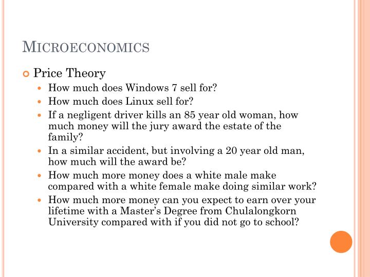
1. Microeconomics • Price Theory • How much does Windows 7 sell for? • How much does Linux sell for? • If a negligent driver kills an 85 year old woman, how much money will the jury award the estate of the family? • In a similar accident, but involving a 20 year old man, how much will the award be? • How much more money does a white male make compared with a white female make doing similar work? • How much more money can you expect to earn over your lifetime with a Master’s Degree from Chulalongkorn University compared with if you did not go to school?

2. Supply & Demand • One of the most persuasive models in the business, social, and behavioral sciences. • Wide applications in fields such as • Economics • Finance • Labor • Statistics • Health • Major Goal: Price Determination.

3. The Law of Demand • An inverse relationship between a measure of price and a measure of the quantity demanded. • As the price of something goes up less of that something is demanded. • What is price? • What is demand?

4. Prices • In microeconomics a price is a ratio that represents terms of trade. • Prices, in micro, are real. • Opportunity costs represent real prices. • In order to get something you have to give something up. • We will use monetary units for convenience. Thus Baht or Dollars represent a medium of exchange…dollars per shirt or dollars per baht represent the price of shirts (in $’s) or the price of baht (in $’s).

5. A Model • Maybe your first economic model was the PPF model…it represents prices in real terms:

6. PPF • In this model we see the terms of trade, i.e., how much Y we get (or give up) when we give up (or get) some amount of X. • Did you notice the curvature of the PPF? It doesn’t need to be this way, but the curve represents increasing marginal cost. That is a standard (and useful assumption): • As we get more X we have to give up increasing amounts of Y.

7. Goods & Services • Production is transformation. • It might be a physical transformation of resources. • It might be a spatial transformation of resources. • It might be a temporal transformation of resources.

8. The Law of Demand • Intuitive. • Applicable to individual decision making. • Applicable to market activity. • Applicable to non-market activity: • Demand for drunk driving. • Demand for quality of life.

9. Demand • Demand exists in the output market. • For example: demand for automobiles. • Demand exists in the input market. • For example: demand for labor. • Some goods & services are both inputs and outputs. • For example: tomatoes.

10. Market Demand • Generated from individual demand. • For example, at a price of 10 baht • Miss Kawita wants 5 units • Mr Chayanin wants 4 units • Mr Satta does not want any units • Miss Utumporn wants 1 unit • At this price 10 units are demanded.

11. Demand may be binary • At a price of Bt 3.95 million (Mercedes E220 CDI) • Richard has zero effective demand – is not in the market • Miss Ungkana has non-zero effective demand – is in the market (do not let BMW know this!) • Aggregation of many zeroes and ones leads to market demand

12. The Law of Demand • Sometimes we can quantify Qd and P • We might model Qd • QdRichard = f(…,P,YRichard, …) • QdRichard = a + bP + cY • b might be -5 • c might be .025 • a represents other determinants

13. Law of Demand • QdRichard = a + bP + cY • This is a linear model and looks like this:

14. Linear Demand • If we examine our demand function holding Y constant (=1000) then we have • Qd = 35 – 5P • This is the same as • P = 7 – Qd/5 • Graphing P against Q – Alfred Marshall

15. P = 7 – Qd/5 • Which Graphs as:

16. Demand as Willingness to Pay • The demand function for an individual represents the maximum amount of money that a person would be willing to pay to purchase a given quantity of a good or service. • The law of demand in this case is a reflection of diminishing marginal utility. • Marginal: incremental.

17. The Supply Function • If I offered to buy all the chocolate chip cookies you brought to class on Saturday for Bt 1000 each, how many cookies would you bring? • If I offered to buy all of the cookies you brought for Bt 2 each, how many would you bring? • In this sense, the Supply Function represents the minimum amount of money a person would be willing to accept to provide a given quantity of a good or service.

18. Supply Preview • Because of the profit motive there is a direct or positive relationship between the quantity supplied of a good or service and its price. • We might model this like: • Qs = f(…, P, …) • Qs = 10P, for example.

19. Equilibrium • When we have a demand function (Qd) and a supply function (Qs) we can think about the price (P) which equilibrates Qd and Qs. This is Pe. • Typically when an observed price Po is greater than Pe we see excess supply and when Po < Pe we have excess demand. Does this make sense to you?

20. Qd = 10 – P; Qs = P; Pe = 5

21. In Labor Economics • There is a demand for labor by firms and there is a supply of labor by households. • The price of labor is the wage. • The demand for labor depends on what sorts of things? • The supply of labor depends on what sorts of things?

22. Wage Determination • As we will see, the demand for labor is called a derived demand. As more consumers want a particular good or service that creates demand for labor in the industry that produces that particular good or service. • What is We in a particular industry?

23. Commodification of Labor • Note that it is theoretically easy to treat labor as we would any other classical input into production such as tomatoes, steel, seeds, or capital. • In the course of your studies you might want to think about this from time to time.

24. Labor • How mobile is labor? • Do prevailing wages adjust to excess supply or demand for labor? • Can certain kinds of labor easily be discriminated against? • What important institutions influence labor supply and/or labor demand decisions?

25. From Here Where? • Now that we have previewed some aspects of micro theory we will explore methods used to model demand and supply functions. • What goes on behind the demand function? • What goes on behind the supply function?

26. From Here… • Price determination might be a reflection of optimal decision making by consumers and producers. • Micro theory can be used as a guide: • Descriptive models of behavior • Prescriptive models of behavior • Ethical Models • Optimal Models

27. Step One • We build are skills by first looking at the demand function. • We will need a few mathematical tools to help us understand how the demand function expresses optimal consumer choice. • Consumers choose among baskets of commodities in order to maximize utility subject to budgetary constraints.

28. Step Two • After we derive the demand function we will do similar exercises for the firm – to discover how the supply function represents maximal profit decision making. • The model is a bit asymmetrical, as we will see.

29. Steps Three, Four, … • Once we are familiar with the basics of supply & demand • What are industries? • What is meant by economic welfare? • When do markets work and when do markets fail? • How would we measure failure? • When is their a role for government?

30. Calculus • Derivatives measure the slopes of lines. • For example, curves do not have slopes, but lines tangent to curves do. • Notice something about curves that have peaks and troughs: • At the peaks and the troughs, the lines tangent at these points have zero slope.

31. First Order Conditions • Finding where the derivatives are equal to zero constitute the first order conditions for maxima and/or minima of functions.

32. Second Order Conditions • If we find a candidate for a maximum or a minimum, how do we tell? • SOC’s help us determine if we have found a max, a min, or something else. • Why are we doing this when we could just graph it? • Multiple dimensions • Econometric specification

33. Calculus • Now watch this example…after the presentation we will slow down and learn how to use the rules of calculus. We will have many simple examples and lots of practice problems.

34. f(x) = x3 - .25x2 – 3x + 3

35. f’(x) = 3x2 – .5x - 3

36. f’(x) = 3x2 – .5x - 3 • At x = 1.0868 f’(x) = 0 • At x = -0.9201 f’(x) = 0 • These are called the critical values of f(x). • Note that at 1.0868 , f(x) reaches what we call a local minimum. • At -0.9201, f(x) reaches a local maximum.

37. f’’(x) = 6x - .5 • At x=1.08, f’’(x) = 6.0279 which is a positive number. • At x=-0.92, f’’(x) = - 6.0279, which is a negative number. • These are examples of FOC and SOC, finding a local min and a local max. • Note f(x) has no global max or min.

38. Examples • f(x) = k • f(x) = ax • f(x) = ax2 + bx + c • f(x) = g(x)*h(x) • f(x) = g(h(x)) • f(x) = g(x)/h(x) • f(x) = ln(x) • f(x) = ex

39. Examples • f(x,y) • Now we have two derivatives • fx and fy which are called partial derivatives • f(x,y) = axy + by2 + c • fx = ay • fy = ax + 2by • FOC’s involve a simultaneous system of equations to solve: • fx = 0 • fy = 0

40. f(x,y) = 3x2 + 2y2

41. f(x,y) = 3x2 + 2y2 • Here, fx = 6x and fy = 4y • At the point (0,0) both of these equations are equal to zero. • Thus (0,0) is a critical value and we see that (0,0) is associated with a minimum value of our objective function

42. f(x,y) = 3x2 – 2y2

43. f(x,y) = 3x2 – 2y2 • For this function there is one critical value, again at (x,y) = (0,0). • But note that this is not associated with a max or a min. • It is called a saddle point.

44. Great News • In this class (and in other econ classes you will take) the functions you deal with will be nicely behaved. • By nicely behaved we mean that we can easily find critical values. • And these critical values will be associated with maximum or minimum values.

45. Forest for Trees • Let’s also remember something important. We do not want to get bogged down in the details of mathematics and forget why we are doing calculus in the first place! • At our level we want to come up with models of prescriptive (optimal) behavior and calculus is tool we use along the way. • Always remember … narrative reasoning is more convincing that equations.