Download
1 / 18
180 likes | 186 Vues
This presentation by Prof. Tadeusz Chrobak from AGH University of Science and Technology in Poland discusses the automation of the generalized curves method for map presentations. It covers the definition and thresholds of curves simplification, smoothing, symbolization, and elimination at different map scales. The presentation also includes examples of open and closed curves generalization and statistics of simplification when map scale changes.

E N D
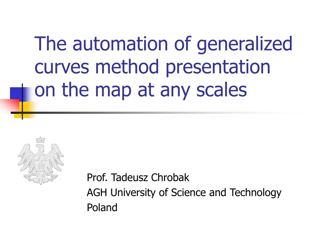
The automation of generalized curves method presentation on the map at any scales Prof. Tadeusz Chrobak AGH University of Science and Technology Poland
The subject of the presentation Definition of curves simplifying parameters, which determine generalization thresholds at any edited map scales, which are: • simplifying, • smoothing, • symbolization, • elimination.
The generalization thresholds distinguishing • In the curves simplifying process conducted by the objective method converted curve maintains statistic distribution properties.
Probability density function of normal – f(x) and normalized – f(u) distribution
The generalization thresholds distinguishing ...continuation Generalization thresholds are definedby dependance: where: n0 – the number of the original curvepoints, ni – the number of points after generalization, c – the number of process invariable points, k – the factor , where k = 1, 2, 3,
The generalization thresholds distinguishing ...continuation • The generalization thresholds can be distinguished depending on standard deviation: • 1 - broken curve simplification, • 2 - curves simplification with smoothing, • 3 - closed curve symbolization or open curve elimination.
No. Scale n0/c Added points Rejected points ni min k=1 k=2 k=3 1 2 3 4 5 6 7 8 9 1 1:1000 133/16 0 0 133 1: 2000 1 1 133 1: 3000 1 1 133 1: 4000 2 2 133 -20 No 1: 5000 16 52 97 7 Yes 1: 6000 12 72 73 25 1:7000 5 83 55 1:8000 1 92 42 1:9000 0 94 39 17 1:10000 1 105 29 0 Yes 1:25000 16 Yes 1:50000 16 1:100000 16 Example
The definition of the generalization method • Objective factors of the method: • drawing recognizability – the elementarytriangle, • points hierarchy, resulting from relative extrema, • added points used to obtain optimal conformity and shapeof generalized curves. • Data accuracy after curves transformation is conserved, apart from scales range.
The definition of the generalization method ...continuation • Conservation of topology and objects classes. • Usefulness for both open and cloesd curves.
Examples • Open curves generalization. • Closed curves generalization. • Statistics of an open curve nodes simplification when map scale is changing from 1:500 to 1:500 000
Open curves generalization, while map scale is changing from 1:500 to 1:2000
Open curves generalization, while map scale is changing from 1:500 to 1:50000
A set of data for the scale Number of nodes Data acquisition M 2 Number of nodes changed removed M5 Number of nodes Changed removed M10 Number of nodes changed removed M25 Number of nodes changed removed M50 Number of nodes changed removed M100 Number of nodes changed removed M200 Number of nodes changed removed M300 Number of nodes changed removed M400 Number of nodes changed removed M500 Number of nodes changed removed M0=1:500 161 nodes source data 159 0 2 117 0 44 74 0 87 29 0 132 17 0 144 9 0 152 4 0 157 3 0 158 3 0 158 2 0 159 M2=1:2000 159 nodes processed data - 117 0 42 74 0 85 29 0 130 17 0 142 9 0 150 4 0 155 3 0 156 3 0 156 2 0 157 M5= 1 : 5000 117 nodes processed data - - 73 1 44 29 0 88 17 0 100 9 1 108 4 0 113 3 0 114 3 0 114 2 0 115 M10= 1 :10000 74 nodes processed data - - - 28 0 46 17 2x 57 9 1 65 4 1 70 3 0 71 3 1 71 2 0 72 M25= 1 :25000 29 nodes processed data - - - - 16 1 13 9 1 20 4 1 25 3 0 26 2 0 27 2 0 27 M50= 1 : 50000 17 nodes processed data - - - - - 8 1 9 4 1 13 3 0 14 2 0 15 2 0 15 M100= 1 : 100000 9 nodes processed data - - - - - - 4 1 5 3 0 6 2 0 7 2 0 7 M200= 1 : 200000 4 nodes processed data - - - - - - - 3 0 1 2 0 2 2 0 2 M300= 1 : 300000 3 nodes processed data - - - - - - - - 2 0 1 2 0 1 M400= 1 : 400000 3 nodes processed data - - - - - - - - - 2 0 1 Statistics of simplification of nodes on an open polygon when map scale is changed from 1:500 to 1:500 000
Conclusions • The open and closed curves (simplified by the objective method) generalization thresholds can be defined by the based on the mathematical statistics method. • The threshold defining correctness is proved bythe conformity of generalization thresholds scales and the maximum of added points scale within 1σ range.