Approximate methods for calculating probability of failure

1. Approximate methods for calculating probability of failure • Working with normal distributions is appealing • First-order second-moment method (FOSM) • Most probable point • First order reliability method (FORM)

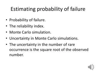
2. The normal distribution is attractive • It has the nice property that linear functions of normal variables are normally distributed. • Also, the sum of many random variables tends to be normally distributed. • Probability of failure varies over many orders of magnitude. • Reliability index, which is the number of standard deviations away from the mean solves this problem.

3. Approximation about mean • Predecessor of FORM called first-order second-moment method (FOSM)

4. Beam under central load example • Probability of exceeding plastic moment capacity • All normal

5. Reliability index for example • Using the linear approximation get • Example 4.2 of CGC shows that if we change to g=T-0.25PL/W we get 3.48 (0.00025, exact is 2.46 or Pf=0.0069)

6. Top Hat question • In the beam example, the error in estimating the reliability index was due to • Linear approximation • g is not normal • both

7. Most probable point (MPP) • The error due to the linear approximation is exacerbated due to the fact that the expansion may be about a point that is far from the failure region (due to the safety margin). • Hasofer and Lind suggested remedying this problem by finding the most probable point and linearizing about it. • The joint distribution of all the random variables assigns a probability density to every point in the random space. The point with the highest density on the line g=0 is the MPP.

8. Response minus capacity illustration r=randn(1000,1)*1.25+10; c=randn(1000,1)*1.5+13; f=@(x) x; fplot(f,[5,20]) hold on plot(r,c,'ro') xlabel('r') ylabel('c')

9. Recipe for finding MPP with independent normal variables • Transform into standard normal variables (zero mean and unity standard deviation) • Find the point on g=0 of minimum distance to origin. The point will be the MPP and the distance to the origin will be the reliability index based on linear approximation there.

10. First order reliability method (FORM) • Limit state g(X). Failure when g<0. • Linear approximation of limit state together with assumption that random variables are normal. • Approximate around most probable point. • Then limit state is also normal variable. • Reliability index is the distance of the mean of g from zero measured in standard deviations.

11. Visual

12. Linear Example • For linear example • Then • The failure boundary • Distance from origin

13. Check by MCS • r=randn(1000,1)*1.25+10; • c=randn(1000,1)*1.5+13; • >> s=0.5*(sign(r-c)+1);pf=sum(s)/1000=0.0550 • Six repetitions gave: 0.0660, 0.0640, 0.0670,0.0450, 0.0550, 0.0640 • With million samples got 0.06258 • So even with a million samples, accurate only to two digits.

14. General case • If random variables are normal but correlated, a linear transformation will transform them to independent variables. • If random variables are not normal, can be transformed to normal with similar probability of failure. See Section 4.1.5 of CGC (It is called the Rosenblatt transformation) • Murray Rosenblatt, Remarks on a Multivariate Transformation, Ann. Math. Statist. Volume 23, Number 3 (1952), 470-472.

15. Approximate transformation • If we want the transformed variable u to have the same CDF as the original x at a certain value of x we would require • Unfortunately we cannot enforce that everywhere. • If we focus on MPP we get the following transformation (Eqs. 4.38, 4.39), which must be used iteratively, starting from some guess. X* replaced by xMPP in equations.