Download
1 / 24
240 likes | 337 Vues
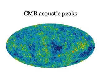
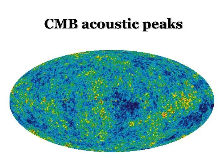
CMB acoustic peaks. Potential fluctuations broken up by mode. hill. well. r, or time. Fluid oscillations in a potential well. Maximum fluid rarification. Maximum velocity – maximum contribution to the Doppler term. Maximum fluid compression. Graphic – Wayne Hu.

E N D
Potential fluctuations broken up by mode hill well r, or time
Fluid oscillations in a potential well Maximum fluid rarification Maximum velocity – maximum contribution to the Doppler term Maximum fluid compression Graphic – Wayne Hu
Potential fluctuations broken up by mode hill well dT/T r, or time baryon-photon fluid propagated this far since Big Bang
3rd acoustic peak fluid compression in potential wells Potential fluctuations broken up by mode hill well dT/T time 2nd acoustic peak fluid compression in potential hills 1st acoustic peak fluid compression in potential wells
Quantitative treatment of oscillations In general, there are three contributions to the observed temperature fluctuations at any given spatial scale smaller than sound horizon, at the time of recombination denser fluid is hotter gravitational redshifting 90 deg out of of phase with the other two
Quantitative treatment of oscillations Gravitational instability: Jeans analysis of small density perturbations in the linear regime (use physical/proper coords) in k-space, differentiating twice is same as multiplying by –k*k assuming Hubble term can be ignored fluid fluid DM general solution why not sin(…) solution? recall continuity eqn. from Jeans analysis: ~ sin(…) will give ~ cos(…) which implies non-0 velocities at t=0 get B by using soln in the oscillator eqn
Quantitative treatment of oscillations Constant A can be obtained by applying the boundary conditions of the Sachs-Wolfe effect, when t is small, or k is small The Doppler velocity term: for a single k-mode
Quantitative treatment of oscillations Putting in values for A and B: The two contributions to temperature (i.e. exlcuding the Doppler term): The velocity Doppler contribution to temperature (multiplied by i, 90deg out of phase) line of sight velocity is a third of full v2
Quantitative treatment of oscillations First, third, etc (odd) acoustic peaks fluid compression in potential wells HOT spots in CMB fluid rarification in potential peaks COLD spots in CMB Second, fourth, etc. (even) acoustic peaks fluid rarification in potential wells COLD spots in CMB fluid compression in potential peaks HOT spots in CMB enhanced by (1+6R) because baryons’ inertia makes them compresses in wells and move away from peaks not enhanced: baryons’ inertia resists rarification in the wells & compression in the peaks Doppler velocity term: amplitude is given by +/- of this amplitude does not change much; baryon-loaded fluid moves slowly
p 2p 3p 4p k (fixed t) k (fixed t) p 2p 3p 4p Potential and Doppler terms; no baryons Potential hill compressions hot spots rarifactions cold spots potential doppler Potential well Sachs-Wolfe effect (small k, large scales)
Add baryons Baryon drag decreases the height of even-numbered peaks (2nd, 4th, etc.) compared to the odd numbered peaks (1st, 3rd, etc.) Potential well 3rd acoustic peak 1st acoustic peak Doppler term is also enhanced, but not as much, because fluid with baryons is heavier, moves slower k (fixed t) p 2p 3p 4p 2nd peak
damping envelope baryon drag WMAP 3 year data Convert +ve and -ve temp. fluctuations to variance in fluctuations, then add grav & thermal + Doppler terms in quadrature 3D -> 2D projection effects and smearing of fluctuations on small scales due to photon diffusion out of structures
Why CMB implies dark matter What we see is the result of baryon-photon fluid oscillations in the potential wells and peaks of dark matter. DM is not directly coupled to baryons & photons. DM density fluctuations have been growing independently of baryons & photons. Need to consider their growth rate first.
Dark matter has no pressure of its own; it is not coupled to photons, so there is almost no restoring pressure force. zero Can assume that total density is the same as critical density at that epoch: Matter dominated epoch: growing decaying mode mode Growth of small DM density perturbations:Sub-horizon, Matter dominated Jeans linear perturbation analysis applies (physical/proper coords): Two linearly indep. solutions: growing mode always comes to dominate; ignore decaying mode soln.
Why CMB implies dark matter Fractional temperature fluctuations in the CMB are ~1/105 The growth rate of density perturbations in the linear regime of non-relativistic component is at most as fast as a=1/(1+z) Recombination took place at z=1000 With no DM, today amplitude of typical fractional overdensities should be 0.01 But, in galaxies and clusters fractional overdensities ~100 and up fluctuations that we see in the CMB are not enough to give us structure today Potential fluctuations at recombination must have been larger than temp. fluct.
Why CMB implies dark matter Evolution of amplitude of a single k-mode Dark matter is not coupled to photons and baryons, so its fluctuations can grow independently. DM fractional overdensities are larger at recombination (but we do not see them directly) Baryon-photon fluid oscillates in the potential wells of DM, but fluctuation amplitude is small – this is what we see as dT/T ~ 1 part in 105. After recombination baryons are let go from photons, and fall into the potential wells of DM. Radiation is free-streaming after recombination. MRE additional x 10-100 log (fractional overdensity) log (scale factor) super-horizon: sub-horizon:
Polarization of the CMB General – applies to primary anisotropy and reionization induced polarization incoming radiation is isotropic; radiation scattered by electron is not polarized incoming radiation is from one direction; radiation scattered by electron is polarized
Polarization of the CMB General – applies to primary anisotropy and reionization induced polarization Needed for polarization: component of radiation where different amplitude of radiation are coming at the electron at 90 degrees between them – this is the property of quarupole distribution
Polarization of the CMB Polarization in the primary anisotropies: single mode potential fluctuation: Where does the quarupole come from during recombination? Convergent velocity field in potential wells/peaks as the fluid oscillates. Then, have to get the projection of these on the plane of the observer’s sky. Most polarization will be seen on scales that correspond to max. fluid velocity – at 90deg from max. fluid compression. Polarization peaks will be between the temperature fluctuation peaks.
Polarization fluctuations Peaks in temp. fluct. correspond to troughs in polarization fluctuations Primary polarization, z~1000 Polarization from the reionization epoch at z~10 Quadrupole radiation field was provided by the CMB primary anisotropies
Measurements of CMBtemperatureand polarization temp-temp auto corr. temp- E pol cross corr. E pol-E pol auto corr B pol-B pol auto corr.