Download
1 / 15
180 likes | 535 Vues
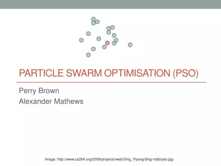
Particle swarm optimisation (PSO). Perry Brown Alexander Mathews. Image: http://www.cs264.org/2009/projects/web/Ding_Yiyang/ding-robb/pso.jpg. Introduction. Concept first introduced by Kennedy and Eberhart (1995)

E N D
Particle swarm optimisation (PSO) Perry Brown Alexander Mathews Image: http://www.cs264.org/2009/projects/web/Ding_Yiyang/ding-robb/pso.jpg
Introduction • Concept first introduced by Kennedy and Eberhart (1995) • Original idea was to develop a realistic visual simulation of bird flock behaviour • Simulation was then modified to include a point in the environment that attracted the virtual bird agents • Potential for optimisation applications then became apparent
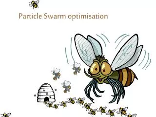
The natural metaphor • A flock of birds (or school of fish, etc.) searching for food • Their objective is to efficiently find the best source of food • Nature-based theory underlying PSO:The advantage of sharing information within a group outweighs the disadvantage of having to share the reward Image: http://www.nerjarob.com/nature/wp-content/uploads/Flock-of-pigeons.jpg
Terminology • The “particles” in PSO have no mass or volume (essentially they are just points in space), but they do have acceleration and velocity • Behaviour of groups in the developed algorithm ended up looking more like a swarm than a flock • Hence the name Particle Swarm Optimisation
Swarm intelligence • Millonas’ five basic principles of swarm intelligence: • Proximity: agents can perform basic space and time calculations • Quality: agents can respond to environmental conditions • Diverse response: population can exhibit a wide range of behaviour • Stability: behaviour of population does not necessarily change every time the environment does • Adaptability: behaviour of population must be able to change when necessary to adapt to environment • A PSO swarm satisfies all of the above conditions
Population and environment • Multidimensional search space • Each point in the search space has some value associated with it, goal is to find the “best” value • Numerous agent particles navigating the search space • Each agent has the following properties: • a current position within the search space • a velocity vector • Additionally, each agent knows the following information: • the best value it has found so far (pbest) and its location • the best value any member of the population has found so far (gbest) and its location
Kennedy and Eberhart’s (1995) refined algorithm • Some number of agent particles are initialised with individual positions and velocities (often just done randomly) • The following steps are then performed iteratively: • The position of each agent is updated according to its current velocity:new position = old position + velocity • The value at each agent’s new position is checked, with pbestand gbest information updated if necessary • Each component of each agent’s velocity vector is then adjusted as a function of the differences between its current location and both the pbest and gbest locations, each weighted by a random variable: new velocity = old velocity + 2 * rand1 * (pbestlocation - current location) + 2 * rand2 * (gbest location - current location)where rand1 and rand2 are random numbers between 0 and 1.(Multiplying by the constant 2 causes particles to “overshoot” their target about half of the time, resulting in further exploration.)
A (partial) example in two dimensions pbests Blue: 0 Green: 0 Red: 0 gbest: 0 (dots indicate agents, yellow star indicates the global optimum)
Begin with random velocities pbests Blue: 0 Green: 0 Red: 0 gbest: 0
Update particle positions pbests Blue: 1 at (6, 2) Green: 0 Red: 2 at (8, 7) gbest: 2 at (8, 7)
Update particle velocities pbests Blue: 1 at (6, 2) Green: 0 Red: 2 at (8, 7) gbest: 2 at (8, 7) For example, Blue’s velocity in the horizontal dimension calculated by:velocity = 1 +2 * rand() * (6 – 6) +2 * rand() * (8 – 6)
Update particle positions again and repeat… pbests Blue: 3 at (8, 6) Green: 1 at (4, 1) Red: 2 at (8, 7) gbest: 3 at (8, 6)
Algorithm termination • The solution to the optimisation problem is (obviously) derived from gbest • Possible termination conditions that might be used: • Solution exceeds some quality threshold • Average velocity of agents falls below some threshold (agents may never become completely stationary) • A certain number of iterations is completed
An example visualisation • http://www.youtube.com/watch?v=_bzRHqmpwvo • Velocities represented by trailing lines • After some individual exploration, particles all converge on global optimum • Particles can be seen oscillating about the optimum
Reference Kennedy, J.; Eberhart, R.; , "Particle swarm optimization," Neural Networks, 1995. Proceedings., IEEE International Conference on , vol.4, no., pp.1942-1948 vol.4, Nov/Dec 1995URL: http://ieeexplore.ieee.org/stamp/stamp.jsp?tp=&arnumber=488968&isnumber=10434