Download
1 / 28
280 likes | 283 Vues
Learning in the brain and in one-layer neural networks. Psychology 209 January 17, 2019. Lecture Outline. Some basic aspects of the neurobiology of learning The Hebb Rule and emergence of patterns in visual cortex Associative learning: Hebbian and error-correcting learning

E N D
Learning in the brain and in one-layer neural networks Psychology 209January 17, 2019
Lecture Outline • Some basic aspects of the neurobiology of learning • The Hebb Rule and emergence of patterns in visual cortex • Associative learning: Hebbian and error-correcting learning • Limitations of the Hebb rule and introduction to error correcting learning – the ‘delta rule’ • Credit assignment with the delta rule, and how the delta rule captures some basic learning phenomena in animal and human learning • Learning in a linear, one-layer network • Introduction to thinking at the level of Patterns • Pattern similarity and generalization • Orthogonality and superposition
The brain is highly plastic and changes in response to experience • Alteration of experience leads to alterations of neural representations in the brain. • What neurons represent, and how precisely they represent it, are strongly affected by experience. • We allocate more of our brain to things we have the most experience with.
Merzenich’s Joined Finger Experiment Controlreceptive fields Receptivefields afterfingers weresown together
Merzenich’s Rotating Disk Experiment: Redistribution and Shrinkage of Fields
Merzenich’s Rotating Disk Experiment: Expansion of Sensory Representation
Synaptic Transmission and Learning Post • Learning may occur by changing the strengths of connections. • Addition and deletion of synapses, as well as larger changes in dendritic and axonal arbors, also occur in response to experience. • New neurons may be added in a specialized sub region of the hippocampus, but there seems to be less of this in the neocortex. Pre
Hebb’s Postulate “When an axon of cell A is near enough to excite a cell B and repeatedly or persistently takes part in firing it, some growth process or metabolic change takes place in one or both cells such that A’s efficiency, as one of the cells firing B, is increased.” D. O. Hebb, Organization of Behavior, 1949 In other words: “Cells that fire together wire together.” Unknown Mathematically, this is often taken as:Dwba = eabaa (Generally you have to subtract something to achieve stability)
b a2 a1
The Molecular Basis of Hebbian Learning (Short Course!) Glutamate ejected fromthe pre-synaptic terminalactivates AMPA receptors,exciting the post-synapticneuron. Glutamate also binds to theNMDA receptor, but it onlyopens when the level of depolarization on the post-synaptic side exceeds a threshold. When the NMDA receptor opens, Ca++ flows in, triggering abiochemical cascade that resultsin an increase in AMPA receptors. The increase in AMPA receptorsmeans that an the same amount of transmitter release at a later time will cause a stronger post-synaptic effect (LTP).
Units 1 & 2 active Unit 3 active alone Final weight .15 .15 .05 How Hebbian Learning Plus Weight Decay Strengthens Correlated Inputs and Weakens Isolated Inputs to a Receiving Neuron unit r 1 2 3input units Activation rule: ar = Ssaswrs Initial weights all = .1 Learning Rule: • Dwrs = earas – d e = 1.0 d = .075 (2x) This works because inputs correlated with otherinputs are associated with stronger activation ofthe receiving unit that inputs that occur on their own.
Miller, Keller, and Stryker (Science, 1989) model ocular dominance column development using Hebbian learning Architecture: • L and R LGN layers and a cortical layer containing 25x25 simple neuron-like units. • Each neuron in each LGN has an initial weak projection that forms a Gaussian hump (illustrated with disc) at the corresponding location in the Cortex, but with some noise around it. • In the cortex, there are short-range excitatory connections and longer-range inhibitory connections, with the net effect as shown in B (scaled version shown next to cortex to indicate approximate scale).
Experience and Training: Before ‘birth’, random activity occurs in each retina. Due to overlapping projections to LGN, neighboring LGN neurons in the same eye tend to be correlated. No (or less) between eye correlation is assumed. Learning of weights to cortex from LGN occurs through a Hebbian learning rule: Dwcl = eacal– decay (Note that w’s are not allowed to go below 0). Results indicate that ocular dominance columns slowly develop over time. Simulation of Ocular DominanceColumn Development based on Hebbian Learning
Associative Learning:e.g. linking what something looks like to how it sounds • Association by contiguity: • If a and b occur together, create a connection between them so that a will activate b • wba = b*a • Generalize by similarity: • If at is similar to al, activate b also. • How do we represent this similarity? • We need to think of a and b as patterns to do so.
Learning Associations: Hebbian vs Error-Driven Learning • Hebb Rule: Dwrs= earas • Here, we force ar to equal the specified output during learning • Delta Rule: Dwrs= e(tr-ar)as • Now, we ‘tell’ the output unit what activation we want it to have • When we test ar= Ssaswrs Our new case: input output + + + + + + + - - -
Credit Assignment, blocking and screening off • Train on tone -> food: • Dog salivates to tone • Train on light -> food: • Dog salivates to light • Blocking:Train with tone -> food,then tone + light => food • Dog does not salivate to light • Division of Labor:Train on tone + light -> food • Dog salivates to tone + light, less to tone or light alone • Screening off:Train on tone + light -> food interleaved with tone -> no food • Dog salivates strongly to light alone,not to tone + light • These patterns can all be explained by the Delta rule! Learnable connections Salivation food tone light Hard-wiredconnection
Associative Learning:e.g. linking what something looks like to how it sounds • Association by contiguity: • If a and b occur together, create a connection between them so that a will activate b (and vice versa): • wba = b*a • Generalize by similarity: • If at is similar to al, activate b also. • How do we represent this similarity? • We need to think of a and b as patterns to do so.
Associating Patterns wrs • Let i and t be patterns of activation, represented by vectors. • We can associate them by creating a weight between each element of i and each element of t. • wrs = etr*is • Diagram shows weights we’d get after applying the above to the patterns shown with e = .125 • red = positive blue = negativePattern input and ‘target’ are always +1 or -1 • ‘output’ is what we get if we multiply the input times the weights or = Ssiswrs Or in vector-matrix notation o = Wi There are details of whether vectors are rows or columns that we are suppressing for now or, tr is
Similarity Relations AmongVectors • Let x and y be vectors of the same length. • Their dot product is the sum of the products of corresponding elements Si xiyi • Their vector correlation or cosine is the extent to which they ‘point in the same direction’. This is often called cos(x,y) Si xiyi /((Si xi xi)½(Siyiyi)½)
Generalization by Similarity • If we’ve associated patterns i and t, and present i’, the output we get will be a scaled version of t: o = tcos(a,a’) • Two patterns are orthogonal if cos(i,i’)=0 • So what output do we get if i and i’ are orthogonal?
Learning Multiple Associationsin the Same set of Weights • We can learn to associate many different i,t pairs in a single pattern associator using the Hebbian learning rule if all of the input patterns are orthogonal: cos(ii,ij)=0 For all pairs of patterns ii, ij (superscripts index patterns) • Targets can be any real vectors. • The weight matrix is just the sum of the weight matrices calculated for each pattern separately. • What happens when a test pattern overlaps with more than one of the patterns used at training?
Learning associations with patterns that are linearly independent but not orthogonal • We can use the ‘Delta rule’ instead of the Hebbian learning rule for learning: Dwrs = (1/n)(tr-or)*is • One can learn arbitrary input-output pairs as long as the input patterns are all linearly independent. That means that none of the input patterns can be expressed as a linear combination of all of the other input patterns. • What happens if one of the inputs can be expressed as a linear combination of the others?
Some Patterns to consider in a one-layer pattern associator • One pattern:a 1.0 -1.0 1.0 -1.0 1.0 -1.0 1.0 -1.0 1.0 1.0 -1.0 -1.0 1.0 1.0 -1.0 -1.0 • Three orthogonal patterns:a 1.0 -1.0 1.0 -1.0 1.0 1.0 -1.0 -1.0 1.0 1.0 -1.0 -1.0 1.0 1.0 -1.0 -1.0 • b 1.0 1.0 -1.0 -1.0 1.0 -1.0 1.0 -1.0 1.0 1.0 1.0 1.0 -1.0 -1.0 -1.0 -1.0 • c 1.0 -1.0 -1.0 1.0 1.0 1.0 1.0 1.0 1.0 -1.0 -1.0 1.0 1.0 -1.0 -1.0 1.0 • Three linearly independent patterns: a 1.0 -1.0 1.0 -1.0 1.0 1.0 -1.0 -1.0 1.0 1.0 -1.0 -1.0 1.0 1.0 -1.0 -1.0 • b 1.0 1.0 -1.0 -1.0 1.0 -1.0 1.0 -1.0 1.0 1.0 1.0 1.0 -1.0 -1.0 -1.0 -1.0 • c 1.0 -1.0 1.0 -1.0 1.0 1.0 1.0 1.0 1.0 -1.0 -1.0 1.0 1.0 -1.0 -1.0 1.0
Learning Central Tendenciesin a Pattern Associator with the Delta Rule • Choose a small learning rate, e.g. 0.0125 • Introduce noise: Each input and output value is perturbed by noise of +/- 0.5 on each training trial • What happens when we repeatedly present noisy examples of a single pattern? • What about interleaved presentations of noisy versions of each of the three orthogonal patterns? • What about the same with the three linearly independent patterns? • What is the effect of learning rate variation? • What happens if we start with a high learning rate and gradually decrease it?
Credit Assignment, blocking and screening off • Train on tone -> food: • Dog salivates to tone • Train on light -> food: • Dog salivates to light • Train with tone -> food,then tone + light => food • Dog does not salivate to light • Train on tone + light -> food • Dog salivates to tone + light, less to tone or light alone • Train on tone + light -> food interleaved with tone -> no food • Dog salivates strongly to light alone • These patterns can all be explained by the Delta rule! Learnable connections Salivation food tone light Hard-wiredconnections