Download
1 / 47
470 likes | 638 Vues
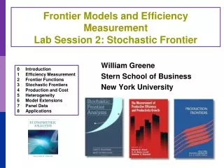
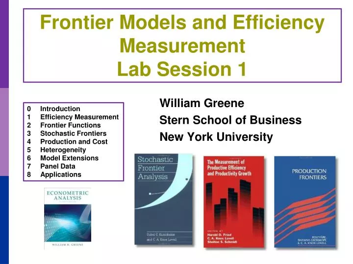
William Greene Stern School of Business New York University. Frontier Models and Efficiency Measurement Lab Session 1. 0 Introduction 1 Efficiency Measurement 2 Frontier Functions 3 Stochastic Frontiers 4 Production and Cost 5 Heterogeneity 6 Model Extensions 7 Panel Data

E N D
William Greene Stern School of Business New York University Frontier Models and Efficiency MeasurementLab Session 1 0 Introduction 1 Efficiency Measurement 2 Frontier Functions 3 Stochastic Frontiers 4 Production and Cost 5 Heterogeneity 6 Model Extensions 7 Panel Data 8 Applications
William Greene Stern School of Business New York University Frontier Models and Efficiency MeasurementLab Session 1: Operating NLOGIT 0 Introduction 1 Efficiency Measurement 2 Frontier Functions 3 Stochastic Frontiers 4 Production and Cost 5 Heterogeneity 6 Model Extensions 7 Panel Data 8 Applications
Lab Session 1 • Operating NLOGIT • Basic Commands - Transformations • Linear Regression/Panel Data Application: Panel data on Spanish Dairy Farms • Estimating the linear model • Testing a hypothesis • Examining residuals
Entering Data for Analysis • IMPORT: ASCII, Excel Spreadsheets, other formats: .txt, .csv, .txt • READ: other programs.dta (stata), .xls (excel) • LOAD existing data sets in the form of LIMDEP/NLOGIT ‘Project Files’ – SAVED from earlier sessions or data preparations.lpj (nlogit, limdep, Stat Transfer) • Internal data editor
Sample data set: dairy.lpj • Panel Data on Spanish Dairy Farms • Use for a Production Function Study • Raw: Milk,Cows,Land, Labor, Feed • Transformed • yit = log(Milk) • x1, x2, x3, x4 = logs of inputs • x11 = .5*x12, x12 = x1*x2, etc. • year93 = dummy variable for year,…
Data on Spanish Dairy Farms N = 247 farms, T = 6 years (1993-1998)
Project Window Project window displays the data set currently being analyzed: Variables Matrices Other program related results
Instructing LIMDEP to do something • Menus – available but we will generally not use them • Command language – entered in an editor then ‘submitted’ to the program
Text Editing Window Commands will be entered in this window and submitted from here
Typing Commands in the Editor Spacing and capitalization never matter. Just type instructions so they are easily readable and contain the right information.
When you open a .lim file, it creates a new editing window for you. Submit the existing commands, modify them then submit, or type new commands in the same window.
“Submitting” Commands • One line command • Place cursor on that line • Press “Go” button • More than one command or command on more than one line • Highlight all lines (like any text editor) • Press “Go” button
The GO Button There is a STOP button also. You can use it to interrupt iterations that seem to be going nowhere. It is red (active) during iterations.
Where Do Results Go? • On the screen in a third window that is opened automatically • In a text file if you request it. • To an Excel CSV file if you EXPORT them • Internally to matrices, variables, etc.
Standard Three Window Operation Commands typed in editing window Project window shows variables in the data set Results appear in output window
Command Structure • VERB ; instruction ; … ; … $ • Verb must be present • Semicolons always separate subcommands • ALL commands end with $ • Case never matters in commands • Spaces are always ignored • Use as many lines as desired, but commands must begin on a new line
Important Commands: • CREATE ; Variable = transformation $ • Create ; LogMilk = Log(Milk) $ • Create ; LMC = .5*Log(Milk)*Log(Cosw) $ • Create ; … any algebraic transformation $ • SAMPLE ; first - last $ • Sample ; 1 – 1000 $ • Sample ; All $ • REJECT ; condition $ • Reject ; Cows < 20 $
Model Command • Model ; Lhs = dependent variable ; Rhs = list of independent variables $ • Regress ; Lhs=Milk ; Rhs=ONE,Feed,Labor,Land $ • ONE requests the constant term - mandatory • Typically many optional variations • Models are REGRESS, FRONTIER, PROBIT, POISSON, LOGIT, TOBIT, … and over 100 others. All have the same form. • Variants of models such as Poisson / NegBinomial • Several hundred different models altogether
Model Command with Sample Definition • Model ; If [ condition ] ; Lhs = … ; Rhs = … ; etc. $ • FRONTIER ; If [Year = 1988] ; Lhs = yit ; Rhs = one,x1,x2,x3,x4 ; Model = Rayleigh $
Name Conventions • CREATE ; Name = any function desired $ • Name is the name of a new variable • No more than 8 characters in a name • The first character must be a letter • May not contain -,+,*,/. • Use letters A – Z, digits 0 – 9 and _ • May contain _.
Two Useful Features NAMELIST ; listname = a group of names $ Listname is any new name. After the command, it is a synonym for the list NAMELIST ; CobbDgls=One,LogK,LogL $ REGRESS ;Lhs = LogY ; Rhs = CobbDgls $ *= All names DSTAT ; RHS = * $ REGRESS ; Lhs = Q ; Rhs = One, LOG* $
A Useful Tool - Calculator CALC ; List ; any expression $ CALC ; List ; 1 + 1 $ CALC ; List ; FTB ( .95,3,1482) $ (Critical point from F table) CALC ; List ; Name = any expression $ Saves result with name so it can be used later. CALC ; Chisq=2*(LogL – Logl0) $ ;LIST may be omitted. Then result is computed but not displayed
Matrix Algebra Large package; integrated into the program. NAMELIST ; X = One,X1,X2,X3,X4 $ MATRIX ; bols = <X’X> * X’y $ CREATE ; e = y – X’bols $ CALC ; s2 = e’e / (N – Col(X)) $ MATRIX ; Vols =s2 * <X’X> ;Stat(bols,Vols,X) $ Over 100 matrix functions and all of matrix algebra are supported. Use with CREATE, CALC, and model estimators.
Regression Results • Model estimates on screen in the output window • Matrices B and VARB • Scalar results • New Variables if requested, e.g., residuals • Retrievable table of regression results
Matrices B and VARB. Double click names to open windows. Use B and VARB in other MATRIX computations and commands.
Scalar results from a regression can also be used in later computations
Regression Analysis: Testing Cobb-Douglas vs. Translog NAMELIST ; cobbdgls = one,x1,x2,x3,x4 $ NAMELIST ; quadrtic =x11,x22,x33,x44,x12,x13,x14,x23,x24,x34 $ NAMELIST ; translog = cobbdgls,quadrtic $ DSTAT ; Rhs=*$ REGRESS ; Lhs = yit ; Rhs = cobbdgls $ CALC ; loglcd = logl ; rsqcd = rsqrd $ REGRESS ; Lhs = yit ; Rhs= translog $ CALC ; logltl = logl ; rsqtl = rsqrd $ CALC ; dfn = Col(translog) – Col(cobbdgls) $ CALC ; dfd = n – Col(translog) $ CALC ; list ; f=((rsqtl – rsqcd)/dfn) / ((1 - rsqtl)/dfd)$ CALC ; list ; cf = ftb(.95,dfn,dfd) $ CALC ; list ; chisq = 2*(logltl – loglcd) $ CALC ; list ; cc = Ctb(.95,dfn) $ Built in F and Chi squared tests REGRESS ; Lhs = yit ; Rhs = translog ; test: quadrtic $
Lab Exercises with Dairy Farm Data • Fit a linear regression with robust covariance matrix • Fit the linear model using least absolute deviations and quantile regression • Test for time effects in the model • Use a Wald test for the translog model • Test for constant returns to scale • Analyze residuals for nonnormality