Download
1 / 36
440 likes | 823 Vues
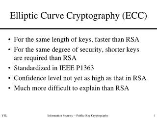
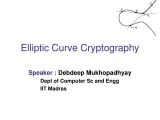
Elliptic Curve Cryptography and Curve Counting Via the Feynman Transform. Michael Slawinski Ph.D. Candidate, UCSD Mathematics Department. Outline. Algebraic Geometry and Cryptography a) Background on Algebraic Geometry i) What is Algebraic Geometry? ii) Algebraic Varieties

E N D
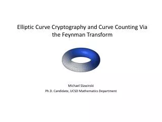
Elliptic Curve Cryptography and Curve Counting Via the Feynman Transform Michael Slawinski Ph.D. Candidate, UCSD Mathematics Department
Outline Algebraic Geometry and Cryptography a) Background on Algebraic Geometry i) What is Algebraic Geometry? ii) Algebraic Varieties iii) Function Fields iv) Divisors v) The Genus of a Curve vi) The Riemann-Roch Theorem vii) The Group Law on the Elliptic Curve b) Elliptic Curve Cryptography II. Thesis project a) The problem b) My contribution and its importance c) Motivation from String Theory d) The project in detail
What is Algebraic Geometry? Algebraic geometry is the study of the relationship between polynomial equations and their solution sets. For example, the solution set of the polynomial equation y = x2 – 1 is given by the parabola y x This equation is rewritten as y – x2 + 1 = 0, and the algebraic variety corresponding to the polynomial f = y – x2 + 1 is the zero set of this polynomial.
Algebraic Varieties An algebraic variety is a set consisting of all roots of a finite collection of polyomial equations with coefficients in a field K : i.e., V(f1, . . . , fm ):= {(x1, . . . , xn)|f1(x1, . . . , xn) = . . . = fm(x1, . . . , xn) = 0} S T ST f = x2 – y – 3 g = x – y + 1 Q h = x – y – 2 P S R V(f,g) = {P, Q} V(f,h) = {R, S} V(f, g, h) = {empty} S = V({fi}) T = V({gj}) ST = V({fi}{gj})
Function Fields The function field K(C) of a curve C, is defined to be the field of rational functions on C. K(C) = { |f and g are polynomial functions on C} Then define K(C)* = {f in K(C) such that fg=1 for some g} . This is the multiplicative group of the function field K(C). K(C) is a vector space over K, where K is the field over which the curve C is defined.
Divisors on Curves A divisor on a curve C is a finite, formal sum of the form D = nPP, where {P} is an arbitrary finite set of points on C and {nP} is a set of integers. The degree of a divisor D, denoted deg D, is nP . C P R Q Some examples of divisors involving these points are D1 = 3P – 4Q + R, D2 = 2P + 13Q – 5R Deg (D1) = 3 – 4 + 1 and deg(D2) = 2 + 13 – 5.
Divisors on Curves Assume that the curve C is smooth, and let f belong to K(C)*. A divisor can be associated to f by defining div(f) = ordP(f) P. For example, let C P R Q We write D 0 if nP 0 for every P in C, and write D1 D2 if D1 – D2 0. Define L(D) = {f in K(C)* such that div(f) – D} {0} and write l(D) for dim L(D). and assume has a zero of order 3 at P, and has a zero of order 2 at R. Then div(f) = 3P – 2R
Divisors on Curves L(D) = {f in K(C)* such that div(f) – D} {0} For example, if D = div(g), then f belongs to L(D) if the numerators of g vanish to higher order than the corresponding poles of f. In other words, fg is defined on the poles of f. Example: If and , then f belongs to L(div(g)) because – 3P – (4P), where P is the origin. Differentials Let C be a curve. The space of meromorphic differential forms on C is a K-vector space generated by symbols of the form dx for x in K(C), subject to the relations: d(x+y) = dx + dy d(xy) = xdy + ydx da = 0 Let be a nonzero differential. Set KC = div().
Genus of a Curve The genus of a curve is a nonnegative integer, which can be defined in any one of the following equivalent ways: • g = dimension of the space of differentials with no poles on C • 2g – 2 = (no. of zeroes) – (no. of poles) of any differential • g = number of handles of C = number of 2-dimensional holes g = 0 g = 1 g = 2
Riemann-Roch Theorem All of these concepts are related in the famous Riemann-Roch Theorem: Let C be a smooth curve. For any divisor D, one has l(D) – l(KC – D) = deg D – g +1, where l(D) = dim L(D) = dim{f in K(C)* such that div(f) – D} {0} This theorem has many applications in algebraic geometry, and in the case of an elliptic curve gives a group structure to the curve itself. This group structure is at the heart of Elliptic Curve Cryptography, or ECC.
The Group Law on an Elliptic Curve An elliptic curve is a smooth, projective algebraic curve of genus one. By the Riemann-Roch theorem, the space L(6[]) has dimension 6, but contains the seven functions 1, x, y, x2, xy, y2, x3. It follows there is a linear relation A1 + A2x + A3y + A4x2 + A5xy + A6y2 + A7x3 = 0 This is the equation of the elliptic curve in the plane.
The Group Law on an Elliptic Curve = O R Q The group law is defined for any three points P, Q, and R by P + Q + R = 0 if and only if P, Q, and R are colinear. The point at infinity O is such that R + (– R) + O = 0. One writes the elliptic curve as (E,O), where E is the curve, and O is the point at infinity. P S
Elliptic Curve Cryptography Let (E,O) be an elliptic curve defined over a finite field Fq where |Fq |= q = pn for p a prime number. Let E(Fq) be the points of E. The Hasse – Weil bound is q + 1 – 2q1/2 |E(Fq)| q + 1 + 2q1/2 The ElGamal elliptic curve cryptosystem is described as follows: Choose a point P in E(Fq) such that it has a large order in the group E(Fq). The curve (E, O) and the point P are public knowledge. The message that Alice wants to send to Bob is assumed to be a point M in E(Fq). Bob chooses an integer d as his private key and publishes Q = dP as his public key. Alice selects a random integer k and computes the points R = kP and S = M + kQ. The pair (R, S) is sent as the ciphertext to Bob. Bob can then recover the plaintext M by computing S + (– d)R. Indeed, S + (– d)R = M + kQ + (– d)R = M + k(dP) + (–d)kP = M. The security of the system is in the difficulty of computing d from dP.
Motivation from String Theory In ten dimensional string theory, the universe consists of the usual four-dimensional Minkowski space time R1,3 , and a “tiny” six-dimensional Calabi-Yau manifold M. The result is the cross product M x R1,3. R1,3 M x {p} p A single fiber of M x R1,3 R1,3
Strings through time and D-branes D1 String at time t + ϵ for ϵ > 0. String at time t D2 The endpoints of the string S are restricted to the D-branes D1 and D2 ,respectively. As S moves through time, it traces out a worldsheet with boundary restricted to D1 and D2.
The problem The space of holomorphic curves on a fixed Calabi-Yau X is denoted Mg,n and consists of all continuous maps from genus g Riemann surfaces to X. For the purposes of this talk, the space Hom(Li, Lj) will be a complex vector space generated by the points of Li Lj, where the Li are special subspaces of the given Calabi-Yau called lagrangians. The counting of holomorphic curves on a Calabi-Yau manifold with boundary on the lagrangian submanifolds is equivalent to expressing the vector space Hom(L0, Ld)[– l][1] Hom(Ld-1, Ld)[– l][-1] Hom(L0, L1) [– l][-1][d – 1+ 2b1] as an algebra over the Feynman transform.
My contribution I have been able to express Hom(L0, Ld)[– l][1] Hom(Ld-1, Ld)[– l][-1] Hom(L0, L1) [– l][-1][d – 1+ 2b1] as an algebra over the Feynman transform in the case that the Calabi-Yau in question is an elliptic curve. FS[t] Hom(L0, Ld)[– l][1] Hom(Ld-1, Ld)[– l][-1] Hom(L0, L1) [– l][-1][d – 1 + 2b1] In other words, there is a linear map of vector spaces encoding special relations among certain elements {md} in the right hand vector space. This type of problem is very important in symplectic geometry, as well as in understanding a phenomenon known as mirror symmetry - the study of ‘mirror’ Calabi-Yau manifolds.
Circle as a quotient of the real line Let R/dZ be the set of real numbers modulo dZ. In other words, x = y in R/dZ if x-y is a multiple of d. This gives R/dZ the topological structure of a circle with circumference d. -2d -d 0 d 2d R projection R/dZ The projection can be visualized as the wrapping of R around R/dZ with each half-open interval [x, x+d) being a cover.
The torus as a fiber bundle Restriction to a single fiber: R C/Z Complex plane Projection Projection R/Z E := C/(Z+Zi)
Lagrangian submanifolds of the torus projection TR L (x,y) (x mod dZ,y) L is given by y = nx. projection A submanifold L M is called lagrangian if ω|TL= 0 and dim L= (1/2) dim M. If M = E is an elliptic curve, then any 1-dimensional submanifold is lagrangian. (x mod dZ,y mod Z) E In the context of the elliptic curve, the lagrangians play the part of the D – branes.
The elliptic curve as a torus The Weierstrass function gives a way of writing the elliptic curve as a 2-torus as opposed to a plane cubic. (z) is defined as follows: C/Z z ((z), ’(z)) y2 = x(x-1)(x- )
The elements ofHom(L0, Ld)[– l][1] Hom(Ld-1, Ld)[– l][-1] Hom(L0, L1) [– l][-1][d – 1 + 2b1] Recall that Hom(Li, Lj) is a complex vector space generated by Li Lj The tensor product AB of two vector spaces A and B is defined as follows AB = {ab| (a1+a2)b = a1b + a2b , and a (b1+b2) = a b1 + a b2 } Using the duality isomorphism Hom(Li, Lj) Hom(Lj, Li)*[l], the elements of Hom(L0, Ld)[– l][1] Hom(Ld-1, Ld)[– l][-1] Hom(L0, L1) [– l][-1][d – 1 + 2b1] can be expressed as maps The elements u are holomorphic maps of the following types:
The holomorphic maps u Complex plane Complex Plane Unit disk in the complex plane L1 p0,1 p1,2 p0,1 L2 L1 p1,0 p0,1 L1 L1 L0 L0 p1,0 p0,2 L p1,2 p1,0 p0,2 L p0,1 L2 L0 L0 nd
Signs of polygons and annuli p0,3 L3 L0 p2,3 p0,1 L2 L1 p1,2 The point p1,2 contributes a +1 as the orientation of L2 agrees with the orientation of C, and p0,3 contributes a -1 as the orientation of L0 disagrees with that of C.
Tropical Morse Graphs-Definition A tropical morse graph is a continuous map (s) from a directed, connected graph G to the circle R/dZ, such that : A vector field ve for each edge e of G, where ve(s) is a tangent vector of R/dZ at (s) Specifically, ve(s) = ve(0) + ne((s) - (0)). 2. The length of e is log(ve(1)/ve(0)). 3. ∑ ve(in)(1) = ∑ ve(out)(0) s e ve(s) (s) The point of the TMG is to provide a combinatorial way of working with the holomorphic maps from disks and annuli to the elliptic curve.
Tropical morse trees R p0,1 p0,1+kd p0,3 p0,3+kd p2,3 p2,3+kd p1,2 p1,2+kd projection p2,3 p1,2 p0,1 p0,3 p2,3 R/dZ Assume maps f to p1,2. The map can either take e to the arc between p2,3 and p1,2 or it can wrap around some integer number of times and then complete this arc. The upshot here is that although the images of the external vertices of T are determined, there are an infinite number of distinct maps , indexed by the integers, which satisfy this. p0,1 p1,2 p0,3
Tropical morse graphs In the graph case, the map does not factor through R as the domain is not simply connected. p0,1 p0,2 p1,2 p0,2 p1,2 p0,1 Note that can still wrap around R/dZ even though there is no lift of to R. The dimension of the space of all maps, Gd, from the space of all graphs with d + 1 external legs, marked by {pi-1,i}, to the circle R/dZ is dim Gd = d – 1 + 2b1 - deg p0,d- deg pi-1,i where b1 is the number of minimal loops of a graph G.
Degeneration of tropical morse trees p2,3 p1,2 p1,3 e(1) e(2) v |e| p1,3 p0,1 e p2,3 p1,2 p0,1 p0,3 Assume (v) is free to move. The tree degenerates when (v) is such that ve(1)(1) + ve(2)(1) = 0. p0,3 The pair of trees on the right corresponds to the composition m2(m2(p2,3, p1,2), p0,1) .
Moduli Space of TMT’s/TMG’s p2,3 p1,2 p1,2 p1,2 p0,1 p2,3 p0,1 p0,1 p2,3 v v v p0,3 p1,2 p0,3 p0,3 p0,1 p2,3 p1,2 p1,2 (v) (v) p0,1 p2,3 (v) p2,3 p0,3 p0,3 p0,1 The point (v) is free to move in R/dZ. In the left-hand picture ve(1)(1) + ve(2)(1) = ve(3)(0), so the length of e(3) is infinite, and the tree degenerates. Similarly for the right-hand picture. As (v) moves around in the circle, the shape of the domain changes accordingly.
Forming polygons/annuli from edges of graphs TR e x [0,1] 0 Lj e x {1} 0 Re s -ve(1) Li e = e x {0} -ve(0) -ve(s) 1 s 1 Re: e x [0,1] TR (s,t) – ni(s) – tve(s) ve(1) ve(s) ve(0)
Polygons swept out by tangent vectors on a single edge Li Li ne= nj - ni e f nf = nj - ni -ve(s) Lj Lj (e) -ve(s) (f)
Polygons correspond to entire graphs p2,3 p1,2 e p0,1 L1 h f L2 L0 v vf k ve vg g w L3 p0,3 p2,3 p1,2 p0,1 p0,3 The balancing conditions at v and w give: i) ve(1) + vh(1) = ve(1) = vf(0) and ii) vf(1) + vk(1) = vf(1) = vg(0)
Relation among md’s, TMT’s/TMG’s p2,3 p1,2 p1,2 p1,2 p0,1 p2,3 p0,1 p2,3 p0,1 |e| = |e| = p0,3 p0,3 p0,3 To each point on this line is associated a TMT with 3 inputs. The endpoints are given by degenerate trees, each of which splits as a composition of two m2’s. Each tree corresponds to a polygon, which in turn gives rise to the sign +1 or – 1. In this case these signs yield the relation m2(m2(p2,3, p1,2), p0,1) m2(p2,3,m2(p1,2, p0,1)) = 0 In the case that b1(G) > 0, these parameter spaces are always 0-dimensional, so there is no relation among the md’s which correspond to graphs with loops.
The result FS[t] These one-dimensional parameter spaces exist for all graphs with b1 = 0, and arbitrarily many legs. Hom(Ld-1, Ld)[– l][1] Hom(Ld-1, Ld)[– l][-1] Hom(L0, L1) [– l][-1][d – 1 + 2b1] The relations among the {md}, resulting from assigning signs to pairs of degenerate trees allows one to define the map of vectors spaces where the basis of the vector space FS[t] can be represented by graphs similar to those already mentioned. The operations {md} corresponding to TMG’s with b1 = 1 satisfy a trivial relation and are described as follows.
The md corresponding to a graph with b1 = 1 FS[t] Hom(Ld-1, Ld)[– l][1] Hom(Ld-1, Ld)[– l][-1] Hom(L0, L1) [– l][-1][d – 1 + 2b1] md where md is given by summing over maps of the form E L p2 p1 L q1 L q2 L L p3 L The annulus wraps around the torus in both directions a finite number of times.
Acknowledgements Thank you to the people of SPAWAR for giving me the opportunity speak about my work, and thank you to my advisor, Professor Mark Gross for suggesting the problem.