Download
1 / 31
330 likes | 538 Vues
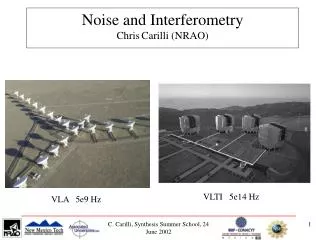
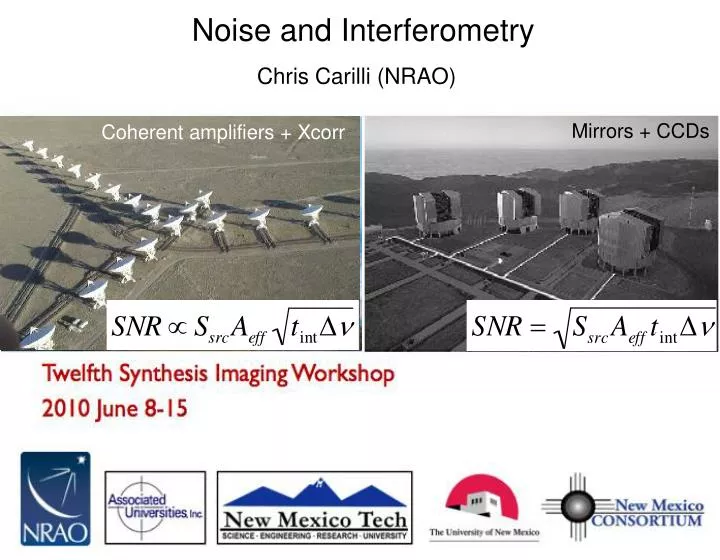
Noise and Interferometry. Chris Carilli (NRAO). Mirrors + CCDs. Coherent amplifiers + Xcorr. References SIRA II (1999) Chapters 9, 28, 33 ‘The intensity interferometer,’ Hanbury-Brown and Twiss 1974 (Taylor-Francis) ‘Letter on Brown and Twiss effect,’ E. Purcell 1956, Nature, 178, 1449

E N D
Noise and Interferometry Chris Carilli (NRAO) Mirrors + CCDs Coherent amplifiers + Xcorr
References • SIRA II (1999) Chapters 9, 28, 33 • ‘The intensity interferometer,’ Hanbury-Brown and Twiss 1974 (Taylor-Francis) • ‘Letter on Brown and Twiss effect,’ E. Purcell 1956, Nature, 178, 1449 • ‘Thermal noise and correlations in photon detection,’ J. Zmuidzinas 2000, Applied Optics, 42, 4989 • ‘Bolometers for infrared and millimeter waves,’ P. Richards, J. 1994, Applied Physics, 76, 1 • ‘Fundamentals of statistical physics,’ Reif (McGraw-Hill) Chap 9 • ‘Tools of Radio Astronomy,’ Rohlfs & Wilson (Springer)
Radiometer Equation (interferometer) • Physically motivate terms • Photon statistics: wave noise vs. shot noise (radio vs. optical) • Quantum noise of coherent amplifiers • Temperature in Radio Astronomy (Johnson-Nyquist resistor noise, Antenna Temp, Brightness Temp) • Number of independent measurements of wave form (central limit theorem) • Some interesting consequences
Concept 1: Photon statistics = Bose-Einstein statistics for gas without number conservation Thermal equilibrium => Planck distribution function (Reif 9.5.4) ns = photon occupation number, relative number in state s = number of photons in standing-wave mode in box at temperature T = number of photons/s/Hz in (diffraction limited) beam in free spacea (Richards 1994, J.Appl.Phys) Photon noise: variance in # photons arriving each second in free space beam (Reif 9.5.6) Optical Radio aConsider TB = Tsys for a diffraction limited beam
‘Bunching of Bosons’: photons can occupy exact same quantum state. Restricting phase space (ie. bandwidth and sampling time) leads to interference within the beam. h h h “Think then, of a stream of wave packetseach about c/ long, in a random sequence. There is a certain probability that two such trains accidentally overlap. When this occurs they interfere and one may find four photons, or none, or something in between as a result. It is proper to speak of interference in this situation because the conditions of the experiment are just such as will ensure that these photons are in the same quantum state. To such interference one may ascribe the ‘abnormal’ density fluctuations in any assemblage of bosons.” (= wave noise) Purcell 1956, Nature, 178, 1449
Photon arrival time Probability of detecting a second photon after interval t in a beam of linearly polarized light with bandwidth (Mandel 1963). Exactly the same factor 2 as in Young 2-slit experiment! 2nd photon knows about 1st Photon arrival times are correlated on timescales ~ 1/, leading to fluctuations total flux, ie. fluctuations are amplified by constructive or destructive interference on timescales ~ 1/ 2nd photon ignorant of 1st Δt
When is wave noise important? • Photon occupation number in CMB (2.7K) • CMB alone is enough to put radio observations into wave noise regime Wien RJ 40GHz
Photon occupation number: examples Bright radio source Optical source Faint radio source Night sky is not dark at radio frequencies!
Wave noise: summary In radio astronomy, the noise statistics are wave noise dominated, ie. noise limit is proportional to the total power, ns, and not the square root of the power, ns1/2
Concept 2: Quantum noise of coherent amplifiers Phase conserving electronics => Δφ < 1 rad Phase conserving amplifier has minimum noise: ns = 1 => puts signal into RJ regime = wave noise dominated. Quantum limit:
Quantum noise: Einstein Coefficients and masers Rohlfs & Wilson equ 11.8 –11.13 Stimluated emission => pay price of spontaneous emission
Consequences: Quantum noise of coherent amplifier (nq = 1) Coherent amplifiers Mirrors + beam splitters Direct detector: CCD Xcorr ‘detection’ ns<<1 => QN disaster, use beam splitters, mirrors, and direct detectors Good: no receiver noise Bad: adding antenna lowers SNR per pair as N2 ns>>1 => QN irrelevant, use phase coherent amplifiers Good: adding antennas doesn’t affect SNR per pair, Polarization and VLBI! Bad: paid QN price
Concept 3: What’s all this about temperatures? Johnson-Nyquist electronic noise of a resistor at TR
Johnson-Nyquist Noise <V> = 0, but <V2> 0 T2 T1 Thermodynamic equil: T1 = T2 • “Statistical fluctuations of electric charge in all conductors produce random variations of the potential between the ends of the conductor…producing mean-square voltage” => white noise power, <V2>/R, radiated by resistor, TR • Analogy to modes in black body cavity (Dickey): • Transmission line electric field standing wave modes: = c/2l, 2c/2l… Nc/2l • # modes (=degree freedom) in + : <N> = 2l / c • Therm. Equipartion law: energy/degree of freedom: <E> ~ kT • Energy equivalent on line in : E = <E> <N> = (kT2l) / c • Transit time of line: t ~l / c • Noise power transferred from each R to line~ E/t = PR = kTR erg s-1
Johnson-Nyquist Noise Thermal noise: <V2>/R = white noise power PR kB = 1.27e-16 +/ 0.17 erg/K TR Noise power is strictly function of TR, not function of R or material.
Antenna Temperature • In radio astronomy, we reference power received from the sky, ground, or electronics, to noise power from a load (resistor) at temperature, TR = Johnson noise • Consider received power from a cosmic source, Psrc • Psrc = Aeff S erg s-1 • Equate to Johnson-Nyquist noise of resistor at TR: PR = kTR • ‘equivalent load’ due to source = antenna temperature, TA: • kTA = Aeff S => TA = Aeff S / k
Brightness Temperature • Brightness temp = surface brightness (Jy/SR, Jy/beam, Jy/arcsec2) • TB = temp of equivalent black body, B, with surface brightness = source surface brightness at : I = S / = B= kTB/ 2 • TB = 2 S / 2 k • TB = physical temperature for optically thick thermal object • TA <= TB always • Source size > beam TA = TBa • Source size < beam TA < TB source TB Explains the fact that temperature in focal plane of telescope cannot exceed TB,src beam telescope a Consider 2 coupled horns in equilibrium, and the fact that TB(horn beam) = Tsys
Radiometry and Signal to Noise Concept 4: number of independent measurements • Limiting signal-to-noise (SNR): Standard deviation of the mean • Wave noise (ns > 1): noise per measurement = (variance)1/2 = <ns> • => noise per measurement total noise power Tsys • Recall, source signal = TA • Inverting, and dividing by signal, can define ‘minimum detectable signal’:
Number of independent measurements How many independent measurements are made by single interferometer (pair ant) for total time, t, over bandwidth, ? Return to uncertainty relationships: Et = h E = h t = 1 t = minimum time for independent measurement = 1/a # independent measurements in t = t/t = t aMeasurements on shorter timescales provide no new information, eg. consider monochromatic signal => t ∞ and single measurement dictates waveform ad infinitum
General Fourier conjugate variable relationships t =1/ • Fourier conjugate variables: frequency – time • If V() is Gaussian of width , then V(t ) is also Gaussian of width = t = 1/ • Measurements of V(t) on timescales t < 1/ are correlated, ie. not independent • Restatement of Nyquist sampling theorem: maximum information on band-limited signal is gained by sampling at t < 1/ 2. Nothing changes on shorter timescales.
Response time of a bandpass filter Vin(t) = (t) Vout(t) ~ 1/ Response of RLC (tuned) filter of bandwidth to impulse V(t) = (t) : decay time ~ 1/. Measurements on shorter timescales are correlateda. Response time: Vout(t) ~ 1/ aclassical analog’ to concept 1 = correlated arrival time of photons
Interferometric Radiometer Equation Interferometer pair: Antenna temp equation: TA = Aeff S / k Sensitivity for interferometer pair: Finally, for an array, the number of independent measurements at give time = number of pairs of antennas = NA(NA-1)/2 Can be generalized easily to: # polarizations, inhomogeneous arrays (Ai, Ti), digital efficiency terms…
Fun with noise: Wave noise vs. counting statistics • Received source power ~ Ssrc × Aeff • Optical telescopes (ns < 1) => rms ~ Nγ1/2 • Nγ SsrcAeff=> SNR = signal/rms (Aeff)1/2 • Radio telescopes (ns > 1) => rms ~ ‘Nγ’ • ‘Nγ’ Tsys = TA + TRx + TBG + Tspill • Faint source: TA << (TRx + TBG + Tspill) => rms dictated by receiver => SNR Aeff • Bright source: Tsys ~ TA SsrcAeff => SNR independent of Aeff
Quantum noise and the 2 slit paradox: wave-particle duality f(τ) Interference pattern builds up even with photon-counting experiment. Which slit does the photon enter? With a phase conserving amplifier it seems one could replace slit with amplifier, and both detect the photon and ‘build-up’ the interference pattern (which we know can’t be correct). But quantum noise dictates that the amplifier introduces 1 photon noise, such that: ns = 1 +/- 1 and we still cannot tell which slit the photon came through!
Intensity Interferometry: ‘Hanbury-Brown – Twiss Effect’ Replace amplifiers with square-law detector (‘photon counter’). This destroys phase information, but cross correlation of intensities still results in a finite correlation! Exact same phenomenon as increased correlation for t < 1/ in photon arrival time (concept 1), ie. correlation of the wave noise itself. • Voltages correlate on timescales ~ 1/ with correlation coef, • Intensities correlate on timescales ~ 1/with correlation coef, Advantage: timescale = 1/ (not 1/) => insensitive to poor optics, ‘seeing’ Disadvantage: No visibility phase information Lower SNR
Interferometric Radiometer Equation • Tsys = wave noise for photons: rms total power • Aeff,kB = Johnson-Nyquist noise + antenna temp definition • t = # independent measurements of TA/Tsys per pair of antennas • NA = # indep. meas. for array
END ESO
Electron statistics:Fermi-Dirac (indistiguishable particles, but number of particles in each state = 0 or 1, or antisymmetric wave function under particle exchange, spin ½)
Quantum limit VI: Heterodyne vs. direct detection interferometry