Download
1 / 29
310 likes | 502 Vues
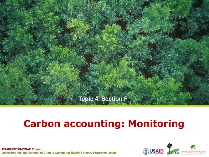
Carbon accounting: Monitoring. Topic 4, Section F. USAID-CIFOR-ICRAF Project Assessing the Implications of Climate Change for USAID Forestry Programs (2009). Learning outcomes. In this presentation you will learn about various monitoring methods for carbon accounting.

E N D
Carbon accounting: Monitoring Topic 4, Section F USAID-CIFOR-ICRAF Project Assessing the Implications of Climate Change for USAID Forestry Programs (2009)
Learning outcomes In this presentation you will learn about various monitoring methods for carbon accounting. Topic 4, Section F, slide 2 of 29
Outline • USAID project monitoring for performance • Data needed for Forest Carbon Calculator • Detailed project monitoring • Monitoring plans • Sampling • Collecting and analyzing data • General concepts and guidance • National monitoring systems • Forest carbon inventory of India • Australian national carbon accounting system • US Forest Service carbon inventory Topic 4, Section F, slide 3 of 29
USAID’s standard climate change indicator • USAID’s standard climate change CO2 indicator: • “Quantity of greenhouse gas emissions, measured in metric tons of CO2 equivalent, reduced or sequestered as a result of USG assistance in natural resources management, agriculture, and/or biodiversity sectors.” • This indicator can be used at the project level with USAID’s Forest Carbon Calculator • If the project is to influence national level policy, the USAID indicator, will be a policy indicator, not CO2 • If USAID engages in large-scale attempts to change a country’s emissions trajectory, then national GHG inventory done with host government provides CO2 impact measures Topic 4, Section F, slide 4 of 29
Data needed for project monitoring with USAID’s Forest Carbon Calculator • Locations of projects according to administrative unit, such as state or district • How many hectares are affected by the activity, such as area of forest protected, reforested, regenerated, or under agroforestry • Measure of project effectiveness: • % reduction in deforestation, • % of trees that survive at end of the year, • % of logging stopped or % of logging that is being done with reduced impact • Documentation of how you estimated project effectiveness measures Topic 4, Section F, slide 5 of 29
Detailed project monitoring • More site-specific monitoring may be desired for project performance or required for carbon finance • Requires a monitoring plan and approach • Monitoring that seeks to measure actual carbon accumulation in soils may be outside the timescale of USAID funding, so measures of activity adoption may be more practical Topic 4, Section F, slide 6 of 29
Manuals and guidebooks • MacDicken (1997) • IPCC GPG (2003) • Pearson et al. (2005) • GOFC-GOLD (2008) Topic 4, Section F, slide 7 of 29
What to monitor? Topic 4, Section F, slide 8 of 29
How to proceed? Define monitoring boundaries (national, project, etc.) Stratify the area to be monitored Decide which carbon pools to measure (5 pools) Determine type, number and location of measurement plots Determine measurement/monitoring frequency Topic 4, Section F, slide 9 of 29
Measuring and monitoring plan for a project-based activity Source: IPCC GPG 2003: Topic 4, Section F, slide 10 of 29
General approach to monitoring • Monitoring carried out through sampling and using existing forest inventory and other data sources • Monitoring should produce estimates of carbon stocks that are both precise and accurate • These will affect the monitoring costs • It is important to design a monitoring system (using stratification, etc.) that produces the desired precision and accuracy with minimal costs (A) Accurate but not precise (B) Precise but not accurate (C) Precise and accurate Topic 4, Section F, slide 11 of 29
Sample size • Calculate the sample size n (number of plots) – based on pre-sampling • Where • n = number of plots to be measured • Syx = estimation error • t = Studet t value • S = variance • X = mean value Topic 4, Section F, slide 12 of 29
Stratification • Allows researchers obtain precise estimates at a lower cost than without stratification • Steps: • Divide heterogeneous population into homogenous groups • Apply monitoring (sampling and calculations) to each strata and compile results at the end Topic 4, Section F, slide 13 of 29
Field plots This schematic diagram represents a three-nest sampling plot in both circular and rectangular forms Source: Pearson et al. 2006 Topic 4, Section F, slide 14 of 29
Frequency of monitoring • For carbon accumulation, the frequency of measurements should be defined in accordance with the rate of change of the carbon stock • Forest processes are generally measured over periods of five-year intervals • Carbon pools that respond more slowly, such as soil, are measured every 10 or even every 20 years • See the graph in the next slide Source: IPCC GPG 2003; Pearson et al. 2005 Topic 4, Section F, slide 15 of 29
Detecting the difference • Two means (time 1 and time 2) • RME = Reliable Minimum Estimate • When number of observations (plots) increases -> variability of the data (standard deviation) decreases • RME 1 is smaller than RME 2 Standard deviation explained A data set with a mean of 50 (shown in blue) and a standard deviation (σ) of 20. Source: IPCC GPG 2003 Topic 4, Section F, slide 16 of 29
Noel Kempff Project (Bolivia): 625 permanent sample plots were measured in 640,000 ha Tons/cell = (tons/ha)*0.0001*(30^2) Vegetation classes Tons of carbon/cell Topic 4, Section F, slide 17 of 29
Noel Kempff (Bolivia) carbon inventory Results based on 625 permanent plots Source: Brown et al., 2000 Topic 4, Section F, slide 18 of 29
Leakage (displacement) • Carbon leakage takes place when interventions to reduce emissions in one geographical area lead to an increase in emissions in another area • Example: if curbing agricultural encroachment into forests in one region results in conversion of forests to agriculture in another region • In the context of REDD, leakage is also referred to as ‘emissions displacement’ • In the Noel Kempff project: • Leakage for the stop-logging component was thoroughly screened and found to be in the 2 to 42% range • Deforestation in local communities actually increased initially, which was hoped to be transitory, related to the creation of new land-use systems Topic 4, Section F, slide 19 of 29
Quality assurance and quality control QA/QC elements: • Reliable field measurements • Re-check measurements with independent crew (10 to 20% of plots re-measured) • Verify laboratory procedures • Re-analyse 10 to 20% of samples • Verify data entry and analysis techniques • Check 10 to15% of the data entries • Adequate data maintenance and archiving • Make sure that data (including computer files, imagery etc.) is adequately achieved Topic 4, Section F, slide 20 of 29
National forest carbon inventory of India • Stratification • The country is stratified into 14 physiographic zones • In each strata, districts are considered first sampling units, 10% of districts are being inventoried every year • Field measurements • National grid and sub-grids are marked as the center of the plot at which a square sample plot of 0.1 hectare is laid out to conduct field inventory of trees • Soil, litter, and humus samples are collected in sub-plots • Carbon calculation • Based on stem volumes obtained in forest inventory • Using expansion factors for conversion from volumes to carbon Topic 4, Section F, slide 21 of 29
Australian National Carbon Accounting System (NCAS) Components: • Remotely sensed land cover change (including mapped information from thousands of satellite images) • Land-use and management data • Climate and soil data • Greenhouse gas accounting tools • Spatial and temporal ecosystem modeling Topic 4, Section F, slide 22 of 29
US Forest Service Carbon Inventory • USDA Forest Inventory and Analysis (FIA) inventory data coupled with a modeling approach • Data from many field plots, collected by FIA beginning in 1950s • Area data from remote sensing • Where FIA data are limited models, such as equations to estimate non-tree carbon are used • System (model) can track carbon through harvested wood products Topic 4, Section F, slide 23 of 29
Large-scale field inventories include remote sensing for area estimation Sample points are located systematically over the effective area and land cover is determined at the point Topic 4, Section F, slide 24 of 29
USDA Forest Inventory Program Evolution • In the recent past, FIA periodically (5-14 years) measured all plots in a state in a 1-2 year timeframe • FIA recently adopted annual inventory, with a subset of plots measured throughout the state each year (5-7 years) • Soil and litter layer carbon measured on subset of plots in new system Topic 4, Section F, slide 25 of 29
US National GHG reporting to UNFCCC • Annual Greenhouse Gas Emissions and Sinks Inventories (1990-present) • US Environmental Protection Agency Topic 4, Section F, slide 26 of 29
Discussion • How should a USAID project set up its monitoring? What fits within its timescale and funding? • Is the accuracy of good measures worth the cost? Topic 4, Section F, slide 27 of 29
References • Brown, S. 1997 Estimating biomass and biomass change of tropical forests: a primer. FAO Forestry Paper no. 134. • Brown, S. 2002 Measuring carbon in forests: current status and futurechallenges Environ. Pollut. 116:363-72. • Brown, S. and Gaston, G. 1995 Use of forest inventories and geographic information systems to estimate biomass density of tropical forests: applications to tropical Africa. Environ. Monit. Assess. 38:157-68. • Brown, S., Hall, M., Andrasko, K., Ruiz, F., Marzoli, W., Guerrero, G., Masera, O., Dushku, A., de Jong, B. and Cornell, J. 2007 Baselines for land-use change in the tropics: application to avoided deforestation projects. Mitigation and Adaptation Strategies for Global Change 12:1001-26. • Brown, S., Burnham, M., Delaney, M., Vaca, R., Powell, M. and Moreno, A. 2000. Issues and challenges for forest-based carbon offset projects: A case study of the Noel Kempff climate action project in Bolivia. Mitigation and Adaptation Strategies for Global Change 5:99-121. • GOFC-GOLD. 2009. Reducing greenhouse gas emissions from deforestation and 46 degradation in developing countries: a sourcebook of methods and procedures 47 for monitoring, measuring and reporting, GOFC-GOLD Report version COP14-2, 48 (GOFC-GOLD Project Office, Natural Resources Canada, Alberta, Canada) • MacDicken, K. G. 1997 A Guide to Monitoring Carbon Storage in Forestry and Agroforestry Projects. Winrock International. • Pearson, T., Walker, S. and Brown, S. 2005 Sourcebook for land use, land-use change and forestry projects. Winrock International and the BioCarbon Fund of the World Bank. 57p. • Penman, J. et al. 2003 Good practice guidance for land use, land-use change and forestry. IPCC National Greenhouse Gas Inventories Program and Institute for Global Environmental Strategies, Kanagawa, Japan. http://www.ipcc-nggip.iges.or.jp/public/gpglulucf/gpglulucf.htm Topic 4, Section F, slide 28 of 29