Download
1 / 15
150 likes | 264 Vues
Aggregate Supply. The AS is the part of our national economy model where the production side is studied. Analogy. Which blade cuts the paper when you use a pair of scissors on the paper? The answer is that you need both to cut the paper.

E N D
Aggregate Supply The AS is the part of our national economy model where the production side is studied.
Analogy Which blade cuts the paper when you use a pair of scissors on the paper? The answer is that you need both to cut the paper. Up to now in our theory about the national economy we have talked about aggregate expenditure, AE, and its connection to aggregate demand, AD. But, just like we need both blades in the scissors, we also have to build in aggregate supply into our theory.
Time Frame As we build a model of the national economy we will need to distinguish between the short run and the long run. (Some of you may have seen the short run and the long run in a micro class. But in this macro class the reason for having both time frames is different than in micro – please note that and try to keep the two straight.) I like to have you think about an analogy to get a feel for the long run and the short run. Imagine that you are running – for now it does not matter what shape you are in, just think about running. When you run right now you have a pace at which you run. The pace is determined by your general health. In a “long run” you will go at your pace.
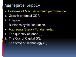
Time Frame For short periods of time you may run faster than the pace – to beat the traffic light or something, or you may run slower than the pace – you know you can not beat the traffic light so you slow down, but still run to keep moving (you are afraid if you quit running you will walk home and never exercise again.) In the long run in the economy there is a natural “pace” for output. That pace is determined by the state of technology and the amount or endowment of resources we have. Long term, the economy will gravitate toward that natural pace. (If you have every jogged you know the pace changes the better shape you are in – and the same is true in the economy.)
Time Frame Another point about the time frame is that the long run is defined as the time frame in which price level changes will be matched by nominal wage and other resource price changes. The short run is defined as the time frame that when the price level changes not enough time has elapsed to permit nominal wage and other resource price changes.
Graph Price level, P Remember we want to use a diagram or graph like this. Let’s see how the long run aggregate supply (LRAS) fits in the graph. RDGP
Long run Given a state of technology and resource endowments the LRAS is shown as one level of RGDP. We place it in the graph at a level – actually determined by looking at real world data. Since it is a vertical line, we see that if the price level should change the quantity supplied in the long run will not change. P LRAS P2 P1 RGDP RGDP1
Long Run The reason the LRAS is a vertical line is because a price level change can not change the level of output – only better technologies or more resources can change the LRAS. In fact, if better technologies or more resources are found the LRAS will shift to the right. So, more labor, capital, natural resources and technological knowledge shift the LRAS to the right. One last point about the LRAS - at any point in history the economy has a potential RGDP level and we show that level as the position of the LRAS. This level of output is called the natural rate of output.
Short Run P LRAS The SRAS has an upward slope to it as we view it from left to right. SRAS P1 RGDP1 RGDP
Short Run On the previous screen you see that at P1 the SRAS = LRAS supply. At prices above P1 we move up the SRAS. How can more be produced in the economy above the natural “pace?” Similarly, at prices below P1 we move down along the SRAS and output would be less than natural. On the last screen the SRAS crossed the LRAS at price level P1. Note that at levels of RGDP less than this the SRAS is somewhat flat and at level of RGDP above this the curve is somewhat steep. Let’s look at this next.
Per unit production cost In order to see the points about SRAS we need to think about the following ratio: Total input cost/units of output. This ratio is the per unit production cost (on average) of output. Ultimately the price per unit has to cover this or firms would not be able to produce. The SRAS is a curve showing what price levels have to be to get the various levels of output produced. When output is already below the full employment level this means many resources are underutilized. So the price level does not have to expand much to get more output. With the higher price level firms have an incentive to produce more.
Per unit production cost Now, when output is already at the full employment level of output or above, additional output is that much harder to come by. In order to get the additions, the price level would have to really jump to get the additional output. Jogging analogy again. When you are jogging really slow you can be induced to speed up with little extra reward, but if you are already sprinting the reward needs to be extra large to get you to go even faster.
Shifting SRAS The SRAS supply curve can shift if we have a change in 1) Input prices, 2) market power, 3) productivity, 4) business taxes and subsidies, and 5) government regulation. Let’s look at each idea here next. If input or resources prices rise, then per unit production costs rise and thus at the same output price level firms in total would reduce output and SRAS would shift to the left. If markets become less competitive firms in those markets that deal with productive resources will have input prices rise, and we have the same result as previously stated.
Shifting SRAS If productivity grows then firms can make available for sale a greater number of goods available for sale at each price level – The SRAS shifts to the right. When business taxes grow, or when subsidies fall, firms have to pay out a greater amount from the price level they receive and therefore they keep less. The fact that they keep less makes them more reluctant to supply and thus SRAS shifts to the left. Government regulation is usually costly for the firm to cover and so more regulations reduce SRAS and this means the curve shifts to the left.
summary In the short run if the price level changes, output can change from the long run level set by technology and resource endowments, but eventually input prices adjust and bring output back in line with the long run pace. We will see later that the time it takes to adjust my be unsatisfactory to you and me. We may want monetary or fiscal policy tools – we discuss later – to “correct” the situation faster.