Download
1 / 56
560 likes | 675 Vues
Modeling of Welding Processes through Order of Magnitude Scaling. Patricio Mendez, Tom Eagar Welding and Joining Group Massachusetts Institute of Technology MMT-2000, Ariel, Israel, November 13-15, 2000. What is Order of Magnitude Scaling?.

E N D
Modeling of Welding Processes throughOrder of Magnitude Scaling Patricio Mendez, Tom Eagar Welding and Joining Group Massachusetts Institute of Technology MMT-2000, Ariel, Israel, November 13-15, 2000
What is Order of Magnitude Scaling? • OMS is a method useful for analyzing systems with many driving forces
What is Order of Magnitude Scaling? • OMS is a method useful for analyzing systems with many driving forces Weld pool
What is Order of Magnitude Scaling? • OMS is a method useful for analyzing systems with many driving forces Weld pool Arc
What is Order of Magnitude Scaling? • OMS is a method useful for analyzing systems with many driving forces Weld pool Arc Electrode tip
Outline • Context of the problem • Simple example of OMS • Applications to Welding • Discussion
Context of the Problem Engineering Science Arts Philosophy
Context of the Problem Engineering Engineering ~1700 Science Science Arts Philosophy Arts Philosophy
Context of the Problem Applications Engineering ~1900 Engineering Engineering ~1700 Science Fundamentals Science Science Arts Philosophy Arts Philosophy
Context of the Problem Applications ~1980 Engineering Gap is getting too large! ~1900 Engineering Engineering ~1700 Science Science Science Arts Philosophy Arts Philosophy Fundamentals
Example: Modeling of an Electric Arc It is very difficult to obtain general conclusions with too many parameters • Very complex process: • Fluid flow (Navier-Stokes) • Heat transfer • Electromagnetism (Maxwell)
Example: Modeling of an Electric Arc Complexity of the physics increased substantially
Generalization of problems with OMS Fundamentals
Generalization of problems with OMS Differential equations Fundamentals
Generalization of problems with OMS Asymptotic analysis (dominant balance) Differential equations Fundamentals
Generalization of problems with OMS Engineering Asymptotic analysis (dominant balance) Differential equations Fundamentals
Generalization of problems with OMS Engineering Dimensional analysis Asymptotic analysis (dominant balance) Differential equations Fundamentals
Generalization of problems with OMS Engineering Dimensional analysis Matrix algebra Asymptotic analysis (dominant balance) Differential equations Fundamentals
Generalization of problems with OMS Engineering Artificial Intelligence Dimensional analysis Matrix algebra Asymptotic analysis (dominant balance) Differential equations Fundamentals
Generalization of problems with OMS Engineering Artificial Intelligence Dimensional analysis Order of Magnitude Reasoning Matrix algebra Asymptotic analysis (dominant balance) Differential equations Fundamentals
Generalization of problems with OMS Engineering Artificial Intelligence Dimensional analysis Order of Magnitude Reasoning Matrix algebra Order of Magnitude Scaling Asymptotic analysis (dominant balance) Differential equations Fundamentals
OMS: a simple example • X = unknown • P1, P2 = parameters (positive and constant)
Dimensional Analysis in OMS • There are two parameters: P1and P2: • n=2
Dimensional Analysis in OMS • There are two parameters: P1and P2: • n=2 • Units of X, P1, and P2 are the same: • k=1 (only one independent unit in the problem)
Dimensional Analysis in OMS • There are two parameters: P1and P2: • n=2 • Units of X, P1, and P2 are the same: • k=1 (only one independent unit in the problem) • Number of dimensionless groups: • m=n-k • m=1 (only one dimensionless group) • P=P2/P1 (arbitrary dimensionless group)
Asymptotic regimes in OMS • There are two asymptotic regimes: • Regime I: P2/P1 0 • Regime II: P2/P1
Dominant balance in OMS • There are 6 possible balances • Combinations of 3 terms taken 2 at a time:
balancing dominant secondary Dominant balance in OMS • There are 6 possible balances • Combinations of 3 terms taken 2 at a time: • One possible balance:
balancing dominant secondary Dominant balance in OMS • There are 6 possible balances • Combinations of 3 terms taken 2 at a time: • One possible balance:
balancing dominant secondary Dominant balance in OMS • There are 6 possible balances • Combinations of 3 terms taken 2 at a time: • One possible balance: P2/P1 0 in regime I
balancing dominant secondary Dominant balance in OMS • There are 6 possible balances • Combinations of 3 terms taken 2 at a time: • One possible balance: XP1 in regime I P2/P1 0 in regime I
balancing dominant secondary Dominant balance in OMS • There are 6 possible balances • Combinations of 3 terms taken 2 at a time: • One possible balance: “natural” dimensionless group XP1 in regime I P2/P1 0 in regime I
Properties of the natural dimensionless groups (NDG) • Each regime has a different set of NDG • For each regime there are m NDG • All NDG are less than 1 in their regime • The edge of the regimes can be defined by NDG=1 • The magnitude of the NDG is a measure of their importance
Estimations in OMS • For the balance of the example: • In regime I: estimation
Corrections in OMS Corrections • Dimensional analysis states: correction function
Corrections in OMS Corrections • Dimensional analysis states: • Dominant balance states: correction function when P2/P10
Corrections in OMS Corrections • Dimensional analysis states: • Dominant balance states: • Therefore: correction function when P2/P10 when P2/P10
Properties of the correction functions Properties of the correction functions • The correction function is 1 near the asymptotic case • The correction function depends on the NDG • The less important NDG can be discarded with little loss of accuracy • The correction function can be estimated empirically by comparison with calculations or experiments
Generalization of OMS • The concepts above can be applied when: • The system has many equations • The terms have the form of a product of powers • The terms are functions instead of constants • In this case the functions need to be normalized
Application of OMS to the Weld Pool at High Current • Driving forces: • Gas shear • Arc Pressure • Electromagnetic forces • Hydrostatic pressure • Capillary forces • Marangoni forces • Buoyancy forces • Balancing forces • Inertial • Viscous
Application of OMS to the Weld Pool at High Current • Governing equations, 2-D model (9) : • conservation of mass • Navier-Stokes(2) • conservation of energy • Marangoni • Ohm (2) • Ampere (2) • conservation of charge
Application of OMS to the Weld Pool at High Current • Governing equations, 2-D model (9) : • conservation of mass • Navier-Stokes(2) • conservation of energy • Marangoni • Ohm (2) • Ampere (2) • conservation of charge • Unknowns (9): • Thickness of weld pool • Flow velocities (2) • Pressure • Temperature • Electric potential • Current density (2) • Magnetic induction
Application of OMS to the Weld Pool at High Current • Parameters (17): • L, r, a, k, Qmax, Jmax, se, g, n, sT, s, Pmax, tmax, U, m0, b, ws • Reference Units (7): • m, kg, s, K, A, J, V • Dimensionless Groups (10) • Reynolds, Stokes, Elsasser, Grashoff, Peclet, Marangoni, Capillary, Poiseuille, geometric, ratio of diffusivity
Application of OMS to the Weld Pool at High Current • Estimations (8): • Thickness of weld pool • Flow velocities (2) • Pressure • Temperature • Electric potential • Current density in X • Magnetic induction
T* d* U* Application of OMS to the Weld Pool at High Current
gas shear / viscous inertial / viscous electromagnetic / viscous convection / conduction Marangoni / gas shear arc pressure / viscous hydrostatic / viscous buoyancy / viscous capillary / viscous diff.=/diff.^ Application of OMS to the Weld Pool at High Current Relevance of NDG (Natural Dimensionless Groups)
Application of OMS to the Arc • Driving forces: • Electromagnetic forces • Radial • Axial • Balancing forces • Inertial • Viscous
Application of OMS to the Arc • Isothermal, axisymmetric model • Governing equations (6): • conservation of mass • Navier-Stokes(2) • Ampere (2) • conservation of magnetic field • Unknowns (6) • Flow velocities (2) • Pressure • Current density (2) • Magnetic induction
Application of OMS to the Arc • Parameters (7): • r, m, m0 , RC , JC , h, Ra • Reference Units (4): • m, kg, s, A • Dimensionless Groups (3) • Reynolds • dimensionless arc length • dimensionless anode radius