Download
1 / 71
810 likes | 1.72k Vues
Isotope Hydrology Shortcourse. Residence Time Approaches using Isotope Tracers. Prof. Jeff McDonnell Dept. of Forest Engineering Oregon State University. Outline. Day 1 Morning: Introduction, Isotope Geochemistry Basics Afternoon: Isotope Geochemistry Basics ‘cont, Examples Day 2

E N D
Isotope Hydrology Shortcourse Residence Time Approaches using Isotope Tracers Prof. Jeff McDonnell Dept. of Forest Engineering Oregon State University
Outline • Day 1 • Morning: Introduction, Isotope Geochemistry Basics • Afternoon: Isotope Geochemistry Basics ‘cont, Examples • Day 2 • Morning: Groundwater Surface Water Interaction, Hydrograph separation basics, time source separations, geographic source separations, practical issues • Afternoon: Processes explaining isotope evidence, groundwater ridging, transmissivity feedback, subsurface stormflow, saturation overland flow • Day 3 • Morning: Mean residence time computation • Afternoon: Stable isotopes in watershed models, mean residence time and model strcutures, two-box models with isotope time series, 3-box models and use of isotope tracers as soft data • Day 4 • Field Trip to Hydrohill or nearby research site
How these time and space scales relate to what we have discussed so far Bloschel et al., 1995
This section will examine how we make use of isotopic variability
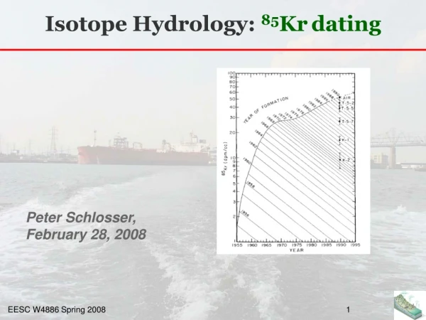
Outline • What is residence time? • How is it determined? modeling background • Subsurface transport basics • Stable isotope dating (18O and 2H) • Models: transfer functions • Tritium (3H) • CFCs, 3H/3He, and 85Kr
Residence time distribution Residence Time • Mean Water Residence Time (aka: turnover time, age of water leaving a system, exit age, mean transit time, travel time, hydraulic age, flushing time, or kinematic age) • tw=Vm/Q • For 1D flow pattern: tw=x/vpw where vpw =q/f • Mean Tracer Residence Time
Why is Residence Time of Interest? • It tells us something fundamental about the hydrology of a watershed • Because chemical weathering, denitrification, and many biogeochemical processes are kinetically controlled, residence time can be a basis for comparisons of water chemistry Vitvar & Burns, 2001
Tracers and Age Ranges • Environmental tracers: • added (injected) by natural processes, typically conservative(no losses, e.g., decay, sorption), or ideal(behaves exactly like traced material)
Modeling Approach • Lumped-parameter models (black-box models): • System is treated as a whole & flow pattern is assumed constant over modeling period • Used to interpret tracer observations in system outflow (e.g. GW well, stream, lysimeter) • Inverse procedure; Mathematical tool: • The convolution integral
Convolution • A convolution is an integral which expresses the amount of overlap of one function h as it is shifted over another function x. It therefore "blends" one function with another • It’s frequency filter, i.e., it attenuates specific frequencies of the input to produce the result • Calculation methods: • Fourier transformations, power spectra • Numerical Integration
Y(w)=F(w)G(w) and • |Y(w)|2=|F(w)| 2 |G(w)| 2 The Convolution Theorem Proof: Trebino, 2002 We will not go through this!!
x(t) g(t) = e -at t g(-t) e -(-at) t e -a(t-t) g(t-t) t x(t)g(t-t) t y(t) Shaded area t t t Multiplication Displacement Folding Integration Convolution: Illustration of how it works Step 1 2 3 4
Example: Delta Function Convolution with a delta function simply centers the function on the delta-function. This convolution does not smear out f(t). Thus, it can physically represent piston-flow processes. Modified from Trebino, 2002
Matrix Set-up for Convolution = [length(x)+length(h)]-1 = length(x) =S y(t) = x(t)*h = 0
Similar to the Unit Hydrograph Precipitation Excess Precipitation Infiltration Capacity Excess Precipitation Time Tarboton
Instantaneous Response Function Unit Response Function U(t) Excess Precipitation P(t) Event Response Q(t) Tarboton
Subsurface Transport Processes • Advection • Dispersion • Sorption • Transformations Modified from Neupauer & Wilson, 2001
Advection Solute movement with bulk water flow t=t1 t2>t1 t3>t2 FLOW Modified from Neupauer & Wilson, 2001
Subsurface Transport Processes • Advection • Dispersion • Sorption • Transformations Modified from Neupauer & Wilson, 2001
Dispersion Solute spreading due to flowpath heterogeneity FLOW Modified from Neupauer & Wilson, 2001
Subsurface Transport Processes • Advection • Dispersion • Sorption • Transformations Modified from Neupauer & Wilson, 2001
Sorption Solute interactions with rock matrix FLOW t2>t1 t=t1 Modified from Neupauer & Wilson, 2001
Subsurface Transport Processes • Advection • Dispersion • Sorption • Transformations Modified from Neupauer & Wilson, 2001
Transformations Solute decay due to chemical and biological reactions MICROBE CO2 t2>t1 t=t1 Modified from Neupauer & Wilson, 2001
Stable Isotope Methods • Seasonal variation of 18O and 2H in precipitation at temperate latitudes • Variation becomes progressively more muted as residence time increases • These variations generally fit a model that incorporates assumptions about subsurface water flow Vitvar & Burns, 2001
Seasonal Variation in 18O of Precipitation Vitvar, 2000
Deines et al. 1990 Seasonality in Stream Water
Cin(t)=A sin(wt) Cout(t)=B sin(wt+j) Example: Sine-wave T=w-1[(B/A)2 –1)1/2
Piston Flow (PFM) • Assumes all flow paths have transit time • All water moves with advection • Represented by a Dirac delta function:
Exponential (EM) • Assumes contribution from all flow paths lengths and heavy weighting of young portion. • Similar to the concept of a “well-mixed” system in a linear reservoir model
Dispersion (DM) • Assumes that flow paths are effected by hydrodynamic dispersion or geomorphological dispersion • Arises from a solution of the 1-D advection-dispersion equation:
Piston flow = Exponential-piston Flow (EPM) • Combination of exponential and piston flow to allow for a delay of shortest flow paths for tT (1-h-1), and g(t)=0 for t< T (1-h-1)
Heavy-tailed Models • Gamma • Exponentials in series
DM DM Exit-age distribution (system response function) Confined aquifer PFM: g(t’) = (t'-T) Unconfined aquifer EM: g(t’) = 1/T exp(-t‘/T) EM EM EPM PFM PFM EM Maloszewski and Zuber Kendall, 2001
DM Exit-age distribution (system response function) cont… • Partly Confined Aquifer: EPM: g(t’) = /T exp(-t'/T + -1) for t‘≥T (1 - 1/) g(t’) = 0 for t'< T (1-1/ ) Kendall, 2001 Maloszewski and Zuber
Review: Calculation of Residence Time • Simulation of the isotope input – output relation: • Calibrate the function g(t) by assuming various distributions of the residence time: • Exponential Model • Piston Flow Model • Dispersion Model
Input Functions • Must represent tracer flux in recharge • Weighting functions are used to “amount-weight” the tracer values according recharge: mass balance!! • Methods: • Winter/summer weighting: • Lysimeter outflow • General equation: where w(t) = recharge weighting function
Model 1 Cin Cout Model 3 g Cin 1- g 1- b Cout Upper reservoir g Model 2 b Direct runoff Cin 1- g Lower reservoir Cout Models of Hydrologic Systems Maloszewski et al., 1983
Soil Water Residence Time Stewart & McDonnell, 2001
Example from Rietholzbach Vitvar, 1998
Model 3… Stable deep signal Uhlenbrook et al., 2002