Engineering Analysis Linear Systems Summary
200 likes | 391 Vues
Engineering Analysis Linear Systems Summary. Yasser F. O. Mohammad. Overview. Convergence criteria of iterative methods Summary of the case M=N Case M>N Case M<N. Strictly Diagonal Matrix. A is said to be strictly diagonal iff. Strictly Diagonal. Not Strictly Diagonal.

Engineering Analysis Linear Systems Summary
E N D
Presentation Transcript
Engineering AnalysisLinear Systems Summary Yasser F. O. Mohammad
Overview • Convergence criteria of iterative methods • Summary of the case M=N • Case M>N • Case M<N
Strictly Diagonal Matrix • A is said to be strictly diagonal iff Strictly Diagonal Not Strictly Diagonal
Jacobi and Gauss Seidel • Jacobi: • Gauss-Seidel
Convergence Criteria • Suppose A is strictly diagonal then: • AX=B has a unique solution X=P • Jacobi Iteration will converge to the solution • Gauss-Seidel Iteration will converge to the solution Is this a necessary or sufficient condition? • In many cases Gauss Seidel will converge FASTER than Jacobi • In some cases Gauss Seidel will NOT converge while Jacobi will
How to determine convergence • Difference between vectors can be measured using metric NORM of the difference vector (X-Y). • Many norms has the form: • P=1 City Blocks Distance • P=2 Euclidean Distance • P=Max absolute Difference
How to do it in matlab • Calculating norm p of X: • (norm(X,p)) • This is defined for p=1,2, ….., • norm(X)==norm(X,2)
Iterative Correction Subtracting (2)-(1) All Known Solving (2) for B Substituting (4) into (3)
How to do Iterative Correction • Do LU factorization to solve AX=B and get the solution X1 (with error) • Calculate B1=AX1-B • Solve AX2=B1 • Now a better estimation of X is X1-X2
Case M>N (Skinny) • Pseudo inverse = • Also called left inverse • This gives the least squares solution which is the solution that minimizes (Not in Exam)
Example (IR=V) • Assume that we measured the voltage and current across a resistor and it was tabulated as: LS solution: 2.202235178041073 Average of the LS error: 0.002235178041072 True value: 2.2 Average of the error: 0.002235178041072
Case M<N (Fat) • AX=B • Cannot have a single solution • Least Norm Solution: • This is the solution with minimum second norm
Doing it in matlab • To find left inverse of A • Ali=inv(A’*A)*A’ • Ali=pinv(A) • To find right inverse of A • Ari=A’*inv(A*A’) • Ari=pinv(A) • To solve for X • X=pinv(A)*B
THE BEST METHOD • Can solve ALL linear systems: • If there is a unique solution it finds it • If there is no solution it reports that • If there are infinite number of solutions it can find them all • Singular Value Decomposition
SVD • Any matrix A (M*N) can be decomposed as: • Where: • U is M*M column orthogonal matrix • S is M*N diagonal matrix!! • V is N*N row orthogonal matrix
Using SVD • Case 1: N=M (Square) • Case 2: M>N (Skinny) • Case 3: M<N (Fat)
Finding SVD in Matlab • [U,S,V]=svd(A) • U*S*V’ A
Easiest way to solve AX=B • Matlab • X=A\B • If N=M Solution • If M>N Least Square Solution • If N>M NOT the Least Norm Solution