Download
1 / 39
390 likes | 546 Vues
Synthesizing High-Frequency Rules from Different Data Sources. Xindong Wu and Shichao Zhang IEEE TRANSACTIONS ON KNOWLEDGE AND DATA ENGINEERING, VOL. 15, NO. 2, MARCH/APRIL 2003. Pre-work. Knowledge management. Knowledge discovery Data mining. Data warehouse. Knowledge Management.

E N D
Synthesizing High-Frequency Rules fromDifferent Data Sources Xindong Wu and Shichao Zhang IEEE TRANSACTIONS ON KNOWLEDGE AND DATA ENGINEERING, VOL. 15, NO. 2, MARCH/APRIL 2003
Pre-work • Knowledge management. • Knowledge discovery • Data mining. • Data warehouse
Knowledge Management • Building data warehousing by Knowledge management
Knowledge Discovery and Data Mining • Data mining is a tool of knowledge discovery
Simon Why data mining If a supermarket manager, simon, want to arrange these commodities into supermarket, how to do will make more revenues, conveniences…. if one customer buys milk then he is likely to buy bread, so... Supermarket Commodities
Simon Why data mining Before long, if simon want to send some advertisement letters for customers, how to consider the individual differences is an important task. Mary always buys diapers and milk powders, she may have a baby, so ….
Useful patterns Knowledge and strategy Preprocess data The role of Data mining
Milk Bread Mining association rules IF bread is bought then milk is bought
Mining steps • step1: define minsup and minconf • ex: minsup=50% minconf=50% • step2: find large itemsets • step3: generate association rules
Example Large itemsets
Outline • Introduction • Weights of Data Sources • Rule Selection • Synthesizing High-Frequency Rules Algorithm • Relative Synthesizing Model • Experiments • Conclusion
DB2 DB1 Introduction • Framework ... DBn AB→C A→D B→E AB→C A→D B→E ... AB→C A→D B→E RD1 RD2 RDn GRB • Synthesizing High-Frequency Rules • Weighting • Ranking
Weights of Data Sources • Definition • Di : data sources • Si : set of association rules from Di • Ri : association rule • 3 Steps • Step 1 : union of all Si • Step 2 : assigning each Ri a weight • Step 3 : assigning each Di a weight & normalization
Example • 3 Data Sources (minsupp=0.2, minconf=0.3) • S1 • AB→C with supp=0.4, conf=0.72 • A→D with supp=0.3, conf=0.64 • B→E with supp=0.34, conf=0.7 • S2 • B→C with supp=0.45, conf=0.87 • A→D with supp=0.36, conf=0.7 • B→E with supp=0.4, conf=0.6 • S3 • AB→C with supp=0.5, conf=0.82 • A→D with supp=0.25, conf=0.62
Step 1 • Union of all Si • S’ = {S1, S2, S3} • R1 : AB→C • S1, S3 2 times • R2 : A→D • S1, S2, S3 3 times • R3 : B→E • S1, S2 2 times • R4 : B→C • S2 1 time
3 2 2 1 = 0.25 = 0.375 = 0.125 = 0.25 WR2= WR4= WR3= WR1= 2 + 3 + 2 + 1 2 + 3 + 2 + 1 2 + 3 + 2 + 1 2 + 3 + 2 + 1 Step 2 • Assigning each Ri a weight • R1 • R2 • R3 • R4
Step 3 • Assigning each Di a weight • WD1 • 2*0.25+3*0.375+2*0.25=2.125 • WD2 • 1*0.125+2*0.25+3*0.375=2 • WD3 • 2*0.25+3*0.375=1.625 • Normalization • WD1 2.125/(2.125+2+1.625)=0.3695 • WD2 2/(2.125+2+1.625)=0.348 • WD3 1.625/(2.125+2+1.625)=0.2825
Why Rule Selection ? • Goal • Extracting High-Frequency Rules • Low-Frequency Rules Noise • Solution • If • Num(Ri) / n < • n : data sources, Num(Ri) : frequency of Ri • Then • Rule Ri be wiped out
Rule Selection • Example : 10 Data Sources • D1~D9 : {R1 : X→Y} • D10 : {R1 : X→Y, R2: X1→Y1, …, R11: X10→Y10 } • Let =0.8 • Num(R1) / 10 = 10/10 = 1 • > keep • Num(R2~11) / 10 = 1/10 = 0.1 • < be wiped out • D1~D10 : {R1 : X→Y} • WR1: 10/10=1 WD1~10: 10*1 / 10*10*1 = 0.1 WR1 n Num(R1)
Comparison • Without Rules Selection • WD1~9 0.099 • WD10 0.109 • With Rules Selection • WD1~10 0.1 • From High-Frequency Rules Point of view • Weight Errors • D1~9 |0.1-0.099| 0.001 • D10 |0.1-0.109| 0.009 • Total Error = 0.01
Synthesizing High-Frequency Rules Algorithm • 5 Steps • Step 1 : Rules Selection • Step 2 : Weights of Data Sources • Step 2.1 : union of all Si • Step 2.2 : assigning each Ri a weight • Step 2.3 : assigning each Di a weight & normalization • Step 3 : computing supp & conf of each Ri • Step 4 : ranking all rules by support • Step 5 : output the High-Frequency Rules
An Example • 3 Data Sources • =0.4, minsupp=0.2, minconf=0.3
Step 1 • Rules Selection • R1 : AB→C • S1, S3 2 times • Num(R1) / 3 = 0.66 keep • R2 : A→D • S1, S2, S3 3 times • Num(R2) / 3 = 1 keep • R3 : B→E • S1, S2 2 times • Num(R3) / 3 = 0.66 keep • R4 : B→C • S2 1 time • Num(R4) / 3 = 0.33 wiped out
2 3 2 = 0.29 = 0.42 = 0.29 WR1= WR2= WR2= 2 + 3 + 2 2 + 3 + 2 2 + 3 + 2 Step 2 : Weights of Data Sources • Weights of Ri • Weight of Di • WD1 2*0.29+3*0.42+2*0.29=2.42 • WD2 3*0.42+2*0.29=1.84 • WD3 2*0.29+3*0.42=1.84 • Normalization • WD1 2.42/(2.42+1.84+1.84)=0.3695=0.396 • WD2 1.84/(2.42+1.84+1.84)=0.302 • WD3 1.84/(2.42+1.84+1.84)=0.302
Step 3 • WD1=0.396 • WD2 =0.302 • WD3=0.302 • Computing supp & conf of each Ri • Support • ABC • 0.396*0.4+0.302*0.5=0.3094 • AD • 0.396*0.3+0.302*0.36=0.228 • BE • 0.396*0.34+0.302*0.4=0.255 • Confidence • ABC • 0.396*0.72+0.302*0.82=0.532 • AD • 0.396*0.64+0.302*0.7=0.465 • BE • 0.396*0.7+0.302*0.6=0.458
Step 4 & Step 5 • Ranking all rules by support & output • minsupp=0.2, minconf=0.3 • ABC, BE, AD • Ranking • 1. ABC (0.3094) • 2. BE (0.255) • 3. AD (0.228) • Output – 3 rules • ABC(0.3094, 0.532) • BE (0.255, 0.458) • AD (0.228, 0.465)
Relative Synthesizing Model • Framework Unknown Di Internet journals books Web X→Y conf=0.7 X→Y conf=0.72 X→Y conf=0.68 • Synthesizing • clustering method • roughly method X→Y conf=?
Synthesizing Methods • Physical Meaning • if the confidences irregularly distributed • Maximum synthesizing operator • Minimum synthesizing operator • Average synthesizing operator • if the confidences (X) normal distribution • clustering interval [a, b] • satisfy • 1. P{ a Xb } (m/n) • 2. | b – a | • 3. a, b > minconf.
Clustering Method • 5 Steps • Step 1 : closeness 1 - | confi – confj | • The distance relation table • Step 2 : closeness degree measure • The confidence-confidence matrix • Step 3 : two confidences close enough ? • The confidence relationship matrix • Step 4 : classes creating • [a, b] interval of the confidence of rule X→Y • Step 5 : interval verifying • satisfy the constraints ?
An Example • Assume • rule X→Y • conf1=0.7, conf2=0.72, conf3=0.68, conf4=0.5 conf5=0.71, conf6=0.69, conf7=0.7, conf8=0.91 • 3 parameters • =0.7 • =0.08 • =0.69
Step 1 : Closeness • Example • conf1=0.7, conf2=0.72 • c1, 2= 1 - | conf1 - conf2 | = 1 - |0.70-0.72|=0.98
Step 2 : Closeness Degree Measure • Example
Step 3 : Close Enough ? • Example • =6.9 > 6.9 < 6.9
Step 4 : Classes Creating • Example 1 Class 1 : conf1~3, conf5~7 3 Class 2 : conf4 Class 3 : conf8 2
Step 5 : Interval Verifying • Example • Class 1 • conf1=0.7, conf2=0.72, conf3=0.68, conf5=0.71, conf6=0.69, conf7=0.7 • [min, max] = [conf3, conf2] = [0.68, 0.72] • constraint 1 P{ 0.68 X 0.72 } (6/8) (0.7) • constraint 2 |0.72-0.68| (0.04) < (0.08) • constraint 3 0.68, 0.75 > minconf. (0.65) • In the same way • Class 2 & Class 3 be wiped out • Result X→Y : conf=[0.68, 0.72] • Support ? • In the same way Interval
Roughly Method • Example • R : AB→C • supp1=0.4, conf1=0.72 • supp2=0.5, conf2=0.82 • Maximum • max ( supp (R) )=max (0.4, 0.5)=0.5 • max ( conf (R) )=max (0.72, 0.82)=0.82 • Minimum & Average • min 0.4, 0.72 • avg 0.45, 0.77
Experiments • Time • SWNBS (without rules selection) • SWBRS (with rules selection) • SWNBS > SWBRS • Error • first 20 frequent itemset • Max=0.000065 • Avg=0.00003165
Conclusion • Synthesizing Model • Data Sources known • weighting • Data Sources unknown • clustering method • roughly method
Future works • Sequence pattern • Combine GA and other techniques