Download
1 / 24
480 likes | 1.23k Vues
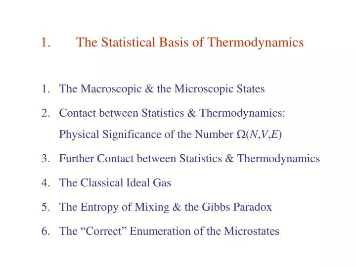
1. The Statistical Basis of Thermodynamics. The Macroscopic & the Microscopic States Contact between Statistics & Thermodynamics: Physical Significance of the Number ( N , V , E ) Further Contact between Statistics & Thermodynamics The Classical Ideal Gas

E N D
1. The Statistical Basis of Thermodynamics The Macroscopic & the Microscopic States Contact between Statistics & Thermodynamics: Physical Significance of the Number (N,V,E) Further Contact between Statistics & Thermodynamics The Classical Ideal Gas The Entropy of Mixing & the Gibbs Paradox The “Correct” Enumeration of the Microstates
1.1. The Macroscopic & the Microscopic States System of N identical particles in volume V, with (Thermodynamic limit ) E.g., Non-interacting particles: i= single particle energies ni = # of p’cles with energy i A macrostate is specified by parameters ( N, V, E, ... ). Postulate of equal a priori probabilities: All microstates satisfying the macrostate parameters are equally likely to occur. Let = # of all microstates that give rise to the macrostate (extensive) parameters N, V, E, ....
1.2. Contact between Statistics & Thermodynamics: Physical Significance of the Number (N,V,E) Consider 2 systems A1 & A2 in thermal contact with each other, i.e., partition is fixed, impermeable but heat conducting. ( Nj , Vj & E(0) = E1 + E2 are fixed ) (0) denotes properties of the composite system A2 ( N2 , V2 , E2 ) A1 ( N1 , V1 , E1 ) Equilibrium is achieved if E1 ( with E2 = E(0) E1) maximizes (0) :
• 2 systems are in thermal equilibrium • if they have the same . Let Thermodynamics : k = Boltzmann constant Boltzmann : 0th law ( thermal eqm.) Planck : 3rd law
1.3. Further Contact between Statistics & Thermodynamics For an impermeable but movable & heat conducting partition, Nj , V(0)= V1 +V2 & E(0) = E1 + E2 are fixed. Equilibrium is achieved, i.e., (0) is maximized, if and i.e., both system have the same values of & 1st law: chemical potential ~ mech. eqm.
For a permeable, movable & heat conducting partition, N(0) = N1 + N2, V(0)= V1 +V2 & E(0) = E1 + E2 are fixed. Equilibrium is achieved, i.e., (0) is maximized, if i.e.,Both system have the same values of ,, & 1st law: ~ chemical eqm.
Summary Connection between statistical mechanics & thermodynamics is Once is written in terms of the independent thermodynamical variables, all other thermodynamic quantities can be obtained via the Maxwell relations.
Mnemonics for the Maxwell Relations Good Physicists Have Studied Under Very Fine Teachers = F ( P) V Y X = H TS G Gibbs free energy T P, Y = U TS F Helmholtz free energy H Enthalpy = U ( P) V Y X V , X S = U(V,S,X) U Internal Energy
1.4. The Classical Ideal Gas Non-interacting, classical ( distinguishable), point particles: const here means indep. of V. Cf
Quantum (Obeying Schrodinger Eq) Free Particles Let these particles be confined within a cube of edge L. Dirichlet boundary conditions: 0 at walls ( where x,y,z = 0,L ). Neumann boundary conditions: n 0 at walls. 1-particle energy :
Let i.e. ( * is a positive integer ) # of { nx, ny, nz} satisfying For N non-interacting particles # of { nix, niy, niz} satisfying
For reversible adiabatic processes, S & N are kept constant. (adiabatic processes) Valid for both classical & quantum statistics
Counting States: Distinguishable Particles State labels { nix, niy, niz} form a lattice in the 3N-D n-space. ( N,E,V)= # of lattice points with non-negative coordinates & lying on the surface of a sphere, centered at the origin, and with radius fluctuates wildly even for small E changes unless N >>1. Better behaved quantity is ( N,E,V), defined as the # of lattice points with non-negative coordinates & lying within the volume bounded by the surface of a sphere, centered at the origin, and with radius
As R , the lattice points become a continuum. ( Density of states in n-space is 1. ) Better approximations: Number of points on the x-y, y-z, z-x planes is Since these pointsare shared by 2 neighboring sectors, the volume integral counts each as half a point. Neumann B.C. (include all nj = 0 points ) Dirichlet B.C. (exclude all nj = 0 points )
( see App.C ) Volume of an n-D sphere of radius R is ( Take non-negative-half of every dimension ) Volume of points with non-negative coordinates
Stirling’s formula: for n>>1 Let (N,V,E) = # of states lying between E ½ & E+ ½ .
Isothermal processes ( N, T = const ) : Adiabatic processes ( N, S = const ) : Alternatively, also leads to
1.5. The Entropy of Mixing & the Gibbs Paradox This S is not extensive, i.e., Thermal wavelength Mixing of 2 ideal gases 1 & 2 (at fixed T ):
Entropy of mixing of gases : Irreversible process: S > 0 is expected. Gibb’s paradox : For the mixing of different parts of the same gas in equilibrium (Ni/ Vi = N / V , i = ), the formula still applies & we also have S > 0, which is unacceptable.
For the mixing of different parts of the same gas in eqm., or Thus, Gibbs’ paradox is resolved using Gibbs’ recipe : Sackur-Tetrodeeq. S is now extensive, i.e.,
Revised Formulae In general, relations derived using the previous definition of S are not modified if they do not involve explicit expression of S. Gibbs’ recipe is cancelled by removing all terms in red. extensive intensive
1.6. The “Correct” Enumeration of the Microstates Elementary particles are all indistinguishable. In the distribution of N particles such that ni particles occupy the i state, for distinguishable particles for indistinguishable particles In the classical (high T ) limit, Gibbs’ recipe corresponds to