Download

1 / 68
680 likes | 876 Vues
Business 260: Managerial Decision Analysis Professor David Mease Lecture 6 Agenda: Go over Midterm Exam 2 solutions 2) Assign Homework #3 (due Thursday 4/23) 3) Reminder: No class Thursday 4/9 4) Data Mining Book Chapter 1 5) Introduction to R 6) Data Mining Book Chapter 4.

E N D
Business 260: Managerial Decision Analysis • Professor David Mease • Lecture 6 • Agenda: • Go over Midterm Exam 2 solutions • 2) Assign Homework #3 (due Thursday 4/23) • 3) Reminder: No class Thursday 4/9 • 4) Data Mining Book Chapter 1 • 5) Introduction to R • 6) Data Mining Book Chapter 4
Homework #3 Homework #3 will be due Thursday 4/23 We will have our last exam that day after we review the solutions The homework is posted on the class web page: http://www.cob.sjsu.edu/mease_d/bus260/260homework.html The solutions are posted so you can check your answers: http://www.cob.sjsu.edu/mease_d/bus260/260homework_solutions.html
No class Thursday 4/9 There is no class this coming Thursday 4/9.
Introduction to Data Mining by Tan, Steinbach, Kumar Chapter 1: Introduction (Chapter 1 is posted at http://www.cob.sjsu.edu/mease_d/bus260/chapter1.pdf)
What is Data Mining? • Data mining is the process of automatically discovering useful information in large data repositories. (page 2) • There are many other definitions
In class exercise #82: Find a different definition of data mining online. How does it compare to the one in the text on the previous slide?
Data Mining Examples and Non-Examples Data Mining: -Certain names are more prevalent in certain US locations (O’Brien, O’Rurke, O’Reilly… in Boston area) -Group together similar documents returned by search engine according to their context (e.g. Amazon rainforest, Amazon.com, etc.) • NOT Data Mining: -Look up phone number in phone directory -Query a Web search engine for information about “Amazon”
Why Mine Data? Scientific Viewpoint • Data collected and stored at enormous speeds (GB/hour) • remote sensors on a satellite • telescopes scanning the skies • microarrays generating gene expression data • scientific simulations generating terabytes of data • Traditional techniques infeasible for raw data • Data mining may help scientists • in classifying and segmenting data • in hypothesis formation
Why Mine Data? Commercial Viewpoint • Lots of data is being collected and warehoused • Web data, e-commerce • Purchases at department/grocery stores • Bank/credit card transactions • Computers have become cheaper and more powerful • Competitive pressure is strong • Provide better, customized services for an edge
In class exercise #83: Give an example of something you did yesterday or today which resulted in data which could potentially be mined to discover useful information.
Origins of Data Mining (page 6) • Draws ideas from machine learning, AI, pattern recognition and statistics • Traditional techniquesmay be unsuitable due to • Enormity of data • High dimensionality of data • Heterogeneous, distributed nature of data AI/Machine Learning/ Pattern Recognition Statistics Data Mining
2 Types of Data Mining Tasks (page 7) • Prediction Methods: Use some variables to predict unknown or future values of other variables. • Description Methods: Find human-interpretable patterns that describe the data.
Examples of Data Mining Tasks • Classification [Predictive] (Chapters 4,5) • Regression [Predictive] (covered in stats classes) • Visualization [Descriptive] (in Chapter 3) • Association Analysis [Descriptive] (Chapter 6) • Clustering [Descriptive] (Chapter 8) • Anomaly Detection [Descriptive] (Chapter 10)
Introduction to R: For the data mining part of this course we will use a statistical software package called R. R can be downloaded from http://cran.r-project.org/ for Windows, Mac or Linux
Reading Data into R Download it from the web at www.stats202.com/stats202log.txt Set your working directory: setwd("C:/Documents and Settings/David/Desktop") Read it in: data<-read.csv("stats202log.txt", sep=" ",header=F)
Reading Data into R Look at the first 5 rows: data[1:5,] V1 V2 V3 V4 V5 V6 V7 V8 V9 1 69.224.117.122 - - [19/Jun/2007:00:31:46 -0400] GET / HTTP/1.1 200 2867 www.davemease.com 2 69.224.117.122 - - [19/Jun/2007:00:31:46 -0400] GET /mease.jpg HTTP/1.1 200 4583 www.davemease.com 3 69.224.117.122 - - [19/Jun/2007:00:31:46 -0400] GET /favicon.ico HTTP/1.1 404 2295 www.davemease.com 4 128.12.159.164 - - [19/Jun/2007:02:50:41 -0400] GET / HTTP/1.1 200 2867 www.davemease.com 5 128.12.159.164 - - [19/Jun/2007:02:50:42 -0400] GET /mease.jpg HTTP/1.1 200 4583 www.davemease.com V10 V11 V12 1 http://search.msn.com/results.aspx?q=mease&first=21&FORM=PERE2 Mozilla/4.0 (compatible; MSIE 7.0; Windows NT 5.1; .NET CLR 1.1.4322) - 2 http://www.davemease.com/ Mozilla/4.0 (compatible; MSIE 7.0; Windows NT 5.1; .NET CLR 1.1.4322) - 3 - Mozilla/4.0 (compatible; MSIE 7.0; Windows NT 5.1; .NET CLR 1.1.4322) - 4 - Mozilla/5.0 (Windows; U; Windows NT 5.1; en-US; rv:1.8.1.4) Gecko/20070515 Firefox/2.0.0.4 - 5 http://www.davemease.com/ Mozilla/5.0 (Windows; U; Windows NT 5.1; en-US; rv:1.8.1.4) Gecko/20070515 Firefox/2.0.0.4 -
Reading Data into R Look at the first column: data[,1] [1] 69.224.117.122 69.224.117.122 69.224.117.122 128.12.159.164 128.12.159.164 128.12.159.164 128.12.159.164 128.12.159.164 128.12.159.164 128.12.159.164 … … … [1901] 65.57.245.11 65.57.245.11 65.57.245.11 65.57.245.11 65.57.245.11 65.57.245.11 65.57.245.11 65.57.245.11 65.57.245.11 65.57.245.11 [1911] 65.57.245.11 67.164.82.184 67.164.82.184 67.164.82.184 171.66.214.36 171.66.214.36 171.66.214.36 65.57.245.11 65.57.245.11 65.57.245.11 [1921] 65.57.245.11 65.57.245.11 73 Levels: 128.12.159.131 128.12.159.164 132.79.14.16 171.64.102.169 171.64.102.98 171.66.214.36 196.209.251.3 202.160.180.150 202.160.180.57 ... 89.100.163.185
Reading Data into R Look at the data in a spreadsheet format: edit(data)
Working with Data in R Creating Data: > aa<-c(1,10,12) > aa [1] 1 10 12 Some simple operations: > aa+10 [1] 11 20 22 > length(aa) [1] 3
Working with Data in R Creating More Data: > bb<-c(2,6,79) > my_data_set<-data.frame(attributeA=aa,attributeB=bb) > my_data_set attributeA attributeB 1 1 2 2 10 6 3 12 79
Working with Data in R Indexing Data: > my_data_set[,1] [1] 1 10 12 > my_data_set[1,] attributeA attributeB 1 1 2 > my_data_set[3,2] [1] 79 > my_data_set[1:2,] attributeA attributeB 1 1 2 2 10 6
Working with Data in R Indexing Data: > my_data_set[c(1,3),] attributeA attributeB 1 1 2 3 12 79 Arithmetic: > aa/bb [1] 0.5000000 1.6666667 0.1518987
Working with Data in R Summary Statistics: > mean(my_data_set[,1]) [1] 7.666667 > median(my_data_set[,1]) [1] 10 > sqrt(var(my_data_set[,1])) [1] 5.859465
Working with Data in R Writing Data: > write.csv(my_data_set,"my_data_set_file.csv") Help!: > ?write.csv
Introduction to Data Mining by Tan, Steinbach, Kumar Chapter 4: Classification: Basic Concepts, Decision Trees, and Model Evaluation (Chapter 4 is posted at http://www.cob.sjsu.edu/mease_d/bus260/chapter4.pdf)
Illustration of the Classification Task: Learning Algorithm Model
Classification: Definition • Given a collection of records (training set) • Each record contains a set of attributes (x), with one additional attribute which is the class (y). • Find a model to predict the class as a function of the values of other attributes. • Goal: previously unseen records should be assigned a class as accurately as possible. • A test set is used to determine the accuracy of the model. Usually, the given data set is divided into training and test sets, with training set used to build the model and test set used to validate it.
Classification Examples • Classifying credit card transactions as legitimate or fraudulent • Classifying secondary structures of protein as alpha-helix, beta-sheet, or random coil • Categorizing news stories as finance, weather, entertainment, sports, etc • Predicting tumor cells as benign or malignant
Classification Techniques • There are many techniques/algorithms for carrying out classification • In this chapter we will study only decision trees • In Chapter 5 we will study other techniques, including some very modern and effective techniques
An Example of a Decision Tree categorical categorical continuous class Splitting Attributes Refund Yes No NO MarSt Married Single, Divorced TaxInc NO < 80K > 80K YES NO Model: Decision Tree Training Data
Applying the Tree Model to Predict the Class for a New Observation Refund Yes No NO MarSt Married Single, Divorced TaxInc NO < 80K > 80K YES NO Test Data Start from the root of tree.
Applying the Tree Model to Predict the Class for a New Observation Refund Yes No NO MarSt Married Single, Divorced TaxInc NO < 80K > 80K YES NO Test Data
Applying the Tree Model to Predict the Class for a New Observation Test Data Refund Yes No NO MarSt Married Single, Divorced TaxInc NO < 80K > 80K YES NO
Applying the Tree Model to Predict the Class for a New Observation Test Data Refund Yes No NO MarSt Married Single, Divorced TaxInc NO < 80K > 80K YES NO
Applying the Tree Model to Predict the Class for a New Observation Test Data Refund Yes No NO MarSt Married Single, Divorced TaxInc NO < 80K > 80K YES NO
Applying the Tree Model to Predict the Class for a New Observation Test Data Refund Yes No NO MarSt Assign Cheat to “No” Married Single, Divorced TaxInc NO < 80K > 80K YES NO
Decision Trees in R • The function rpart() in the library “rpart” generates decision trees in R. • Be careful: This function also does regression trees which are for a numeric response. Make sure the function rpart() knows your class labels are a factor and not a numeric response. (“if y is a factor then method="class" is assumed”)
In class exercise #84: Below is output from the rpart() function. Use this tree to predict the class of the following observations: a) (Age=middle Number=5 Start=10) b) (Age=young Number=2 Start=17) c) (Age=old Number=10 Start=6) 1) root 81 17 absent (0.79012346 0.20987654) 2) Start>=8.5 62 6 absent (0.90322581 0.09677419) 4) Age=old,young 48 2 absent (0.95833333 0.04166667) 8) Start>=13.5 25 0 absent (1.00000000 0.00000000) * 9) Start< 13.5 23 2 absent (0.91304348 0.08695652) * 5) Age=middle 14 4 absent (0.71428571 0.28571429) 10) Start>=12.5 10 1 absent (0.90000000 0.10000000) * 11) Start< 12.5 4 1 present (0.25000000 0.75000000) * 3) Start< 8.5 19 8 present (0.42105263 0.57894737) 6) Start< 4 10 4 absent (0.60000000 0.40000000) 12) Number< 2.5 1 0 absent (1.00000000 0.00000000) * 13) Number>=2.5 9 4 absent (0.55555556 0.44444444) * 7) Start>=4 9 2 present (0.22222222 0.77777778) 14) Number< 3.5 2 0 absent (1.00000000 0.00000000) * 15) Number>=3.5 7 0 present (0.00000000 1.00000000) *
In class exercise #85: Use rpart() in R to fit a decision tree to last column of the sonar training data at http://www-stat.wharton.upenn.edu/~dmease/sonar_train.csv Use all the default values. Compute the misclassification error on the training data and also on the test data at http://www-stat.wharton.upenn.edu/~dmease/sonar_test.csv
In class exercise #85: Use rpart() in R to fit a decision tree to last column of the sonar training data at http://www-stat.wharton.upenn.edu/~dmease/sonar_train.csv Use all the default values. Compute the misclassification error on the training data and also on the test data at http://www-stat.wharton.upenn.edu/~dmease/sonar_test.csv Solution: install.packages("rpart") library(rpart) train<-read.csv("sonar_train.csv",header=FALSE) y<-as.factor(train[,61]) x<-train[,1:60] fit<-rpart(y~.,x) 1-sum(y==predict(fit,x,type="class"))/length(y)
In class exercise #85: Use rpart() in R to fit a decision tree to last column of the sonar training data at http://www-stat.wharton.upenn.edu/~dmease/sonar_train.csv Use all the default values. Compute the misclassification error on the training data and also on the test data at http://www-stat.wharton.upenn.edu/~dmease/sonar_test.csv Solution (continued): test<-read.csv("sonar_test.csv",header=FALSE) y_test<-as.factor(test[,61]) x_test<-test[,1:60] 1-sum(y_test==predict(fit,x_test,type="class"))/ length(y_test)
In class exercise #86: Repeat the previous exercise for a tree of depth 1 by using control=rpart.control(maxdepth=1). Which model seems better?
In class exercise #86: Repeat the previous exercise for a tree of depth 1 by using control=rpart.control(maxdepth=1). Which model seems better? Solution: fit<- rpart(y~.,x,control=rpart.control(maxdepth=1)) 1-sum(y==predict(fit,x,type="class"))/length(y) 1-sum(y_test==predict(fit,x_test,type="class"))/ length(y_test)
In class exercise #87: Repeat the previous exercise for a tree of depth 6 by using control=rpart.control(minsplit=0,minbucket=0, cp=-1,maxcompete=0, maxsurrogate=0, usesurrogate=0, xval=0,maxdepth=6) Which model seems better?
In class exercise #87: Repeat the previous exercise for a tree of depth 6 by using control=rpart.control(minsplit=0,minbucket=0, cp=-1,maxcompete=0, maxsurrogate=0, usesurrogate=0, xval=0,maxdepth=6) Which model seems better? Solution: fit<-rpart(y~.,x, control=rpart.control(minsplit=0, minbucket=0,cp=-1,maxcompete=0, maxsurrogate=0, usesurrogate=0, xval=0,maxdepth=6)) 1-sum(y==predict(fit,x,type="class"))/length(y) 1-sum(y_test==predict(fit,x_test,type="class"))/ length(y_test)
How are Decision Trees Generated? • Many algorithms use a version of a “top-down” or “divide-and-conquer” approach known as Hunt’s Algorithm (Page 152): Let Dt be the set of training records that reach a node t • If Dt contains records that belong the same class yt, then t is a leaf node labeled as yt • If Dt contains records that belong to more than one class, use an attribute test to split the data into smaller subsets. Recursively apply the procedure to each subset.