Download
1 / 17
170 likes | 339 Vues
Local Prediction of a Spatio-Temporal Process with Application to Wet Sulfate Deposition. Presented by Isin OZAKSOY. Benefits of Spatial-Temporal over Spatial :. Use larger sample size to support model estimation Spatio-temporal drift estimates Location- specific forecasts

E N D
Local Prediction of aSpatio-Temporal Process with Application to Wet Sulfate Deposition Presented by Isin OZAKSOY
Benefits of Spatial-Temporal over Spatial : • Use larger sample size to support model estimation • Spatio-temporal drift estimates • Location- specific forecasts • Temporal correlation estimates Goal of article : • Estimate a model of sulfate deposition that captures the major effects of location, time, and season on the mean value and covariance structure • Provide original-scale process predictions and prediction standard error estimates that are both negligibly biased. • Develop a predictor capable of estimating the parameter of a substantive science-based pollutant deposition model.
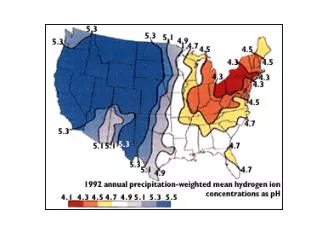
Data : • 5039 seasonal sulfate decomposition • 160 monitoring sites • Summer 1979 – Summer 1992 • Constructing seasonal deposition observations : (percip. mean weighted average of weekly obs.) * (total percip. of season) • Include only observations meeting second-highest data completeness criterion • Note that, seasonal data is less noisy but still can estimate seasonal effect.
Definitions : (x,y) : spatial coordinates of locations in spatio-temporal space t : temporal coordinates X=(x,y,t)’ : spatio-temporal location n : total number of spatio-temporal observations fc : fraction of n used for prediction nc =n* fc : number of observations used to predict at xo Prediction Cylinder : Spatio-temporal space that holds the nc observations used to predict the process at xo . NOTE : Spatial and temporal dimensions of cylinder are defined separately.
Step 1 : mT≤ tlatest - tearliest mT= tU - tL tL = max ( tearliest , tU - mT ) tU = min ( tO , tO + (mT /2) ) nI observations within temp. interval mTlarge enough so nC < nI Step 2 : Sort nI observations according to ||(xO,yO)’ – (x,y)’|| Sort nI observations according to | tO – t | Step 3 : Cylinder`s obs. are first nC of sorted nI observations. Cylinder`s radious : Spatial distance between the nCth observation and (xO,yO)’ Determining Cylinder`s nC Observations tearliest tL tO tU tlatest
Modelling : Spatio-Temporal Drift Model VC : Variance- covariance matrix between residuals at xO and the residuals at the observation locations.
Reasons for using Spatial-Temporal Drift Model : • Sulfate`s spatial drift exhibits an inverted bowl shape centered over the Ohio Valley. • Sulfate deposition exhibits strong seasonality. • Demonstrate feasibility of estimating nonlinear spatio-temporal drift models with MCSTK.
Spatio-Temporal Covariance : • Within Cylinder Covariance Function : E(RC(x)) is constant. Cov(RC(x1), RC(x2))=CS,T(g((x1,y1)’, (x2,y2)’), h(t1,t2)’) where; CS,T(. , .)’ : Spatio-temporal covariance function, g((x1,y1)’, (x2,y2)’) = ||(x1,y1)’ – (x2,y2)’|| : spatial lag h(t1,t2)’ = | t1 – t2 | : temporal lag
Spatio-Temporal Covariance : • Spatio-Temporal Semivariogram Estimation : • Consider all combinations of mS spatial lags and mT+1 temporal lags. • mS is determined to control the pair count per semivariogram estimate (semivar. estimate based on small number of pairs may have high variance). • Nkl is the number of spatio-temporal observation pairs separated by spatio- temporal lag class (gk ,hl ) • where a(.) is the nugget, s(.) is the partial sill and r(.) is the range. To weight semivariogram estimates by their number of pairs per lag class and to give more weight to small semivariogram estimates, use
MCSTK Algorithm (Prediction at xO) STEP 1 : • Set VC= I and Y(m(x,bC),x) = 1 • Compute OLS estimate and • Estimate spatio-temporal semi-variogram model from these residuals and use the covariance function from the estimated semi-variogram to compute STEP 2 : • Set VC= and Y(m(x,bC),x) = 1 • Compute GLS estimate and • Estimate spatio-temporal semi-variogram model from these residuals and use the covariance function from the estimated semi-variogram to compute STEP 3 : • Use covariance function model to predict kriging the residual process at xO via residual kriging.
MCSTK Algorithm (Prediction at xO) w : kriging weights : lagrange multiplier : estimate of UC from covariance function in Step 2
Heteroscedastic Residual Variance Function Estimate ( ) IMPORTANT : Errors must NOT be dependent ! STEP 1 : Find nS observation locations within the cylinder from the same seasonality level and temporally closest to the prediction time. STEP 2 : Sort nS locations by . STEP 3 : Let be sample variance of the second-stage residuals computed at first nn of the sorted locations. Let be sample variance of the second-stage residuals computed at all nS locations. is sample variance of the nn closest residuals to the prediction location in terms of seasonality level, time, and estimated drift. STEP 4 : Calculate the heteroscedasticity function at xO by :
MCSTK Bias Assessment and fC Determination BAIS ASSESSMENT : MCSTK predictor and it's estimated standard error is bias for E(YC(xO)) and se(xO) respectively. Case : If VC is known and RC(x) is homoscedastic, GLS drift estimate is found by finding that minimizes . Define predicted residuals to be . If is known, then the kriging and variance from the residual kriging equations is equal to : PREDICTION BIAS : For i=1,…,nCV define cross-validation residuals and the standardized cross-validation residuals be
MCSTK Bias Assessment and fC Determination PREDICTION BIAS : • Compute mean bias as fraction of data means; where is the mean of nCV observations. • Perform t-test on cross validation residuals of the hypothesis that PREDICTION STANDARD ERROR ESTIMATE BIAS : • If is negligibly bias for but estimated standard error is biased for true prediction standard error then and the sample standard deviation of indicates the direction and degree of the bias in the estimated standard errors. • If estimate standard errors are negligibly bias then where
MCSTK Bias Assessment and fC Determination REASON FOR BIAS IN STANDARD ERROR • As cylinder radius increases, cylinder model for spatial drift captures less of the increasing complicated drift surface which then is represented by residuals which inflates semivariogram estimates (resulting in positive bias). • If cylinder is too small, then the semivariogram estimates in MCSTK is seriously negative biased at larger lags. Since kriging is performed locally, estimated standard errors may not be significantly biased if kriging system's size is not too small. NOTE : Reliability of MCSTK estimated standard errors increases as reliability of semivariogram estimates increases. fC DETERMINATION Cross-validation is performed over a set of fC values and the smallest value of fC values selected for the prediction and standard error estimate bias are as small as possible.
CONCLUSIONS : • MCSTK is flexible for modeling linear and/or nonlinear spatio-temporal process with residual covariance structure. Thus, can do full vs. reduced model analysis. • Data sets from environmental spatio-temporal processes which are first and second order non-stationary can be large enough so with appropriate cylinder size, MCSTK predictions and standard error estimates are negligible and small biased. • For separable spatio-temporal covariance function, ill-conditioned kriging system has inevitable instability. • In the time period 1987-1992, U.S. sulfate deposition decreased over East and West but increased in Southwest, Rocky Mountains and South Texas. • Assumption of zero-temporal covariance minimally effects seasonal sulfate deposition P.I. for this data. • MCSTK is computationally intensive.