Download

1 / 50
520 likes | 709 Vues
Automatic Disease Detection In Citrus Trees Using Machine Vision. Rajesh Pydipati Research Assistant Agricultural Robotics & Mechatronics Group (ARMg) Agricultural & Biological Engineering. Introduction. Citrus industry is an important constituent of Florida’s overall agricultural economy

E N D
Automatic Disease Detection In Citrus Trees Using Machine Vision Rajesh Pydipati Research Assistant Agricultural Robotics & Mechatronics Group (ARMg) Agricultural & Biological Engineering
Introduction • Citrus industry is an important constituent of Florida’s overall agricultural economy • Florida is the world’s leading producing region for grapefruit and second only to Brazil in orange production • The state produces over 80 percent of the United States’ supply of citrus
Research Justification • Citrus diseases cause economic loss in citrus production due to long term tree damage and due to fruit defects that reduce crop size, quality and marketability. • Early detection systems that might detect and possibly treat citrus for observed diseases or nutrient deficiency could significantly reduce annual losses.
Objectives • Collect image data set of various common citrus diseases. • Evaluate the Color Co-occurrence Method, for disease detection in citrus trees. • Develop various strategies and algorithms for classification of the citrus leaves based on the features obtained from the color co-occurrence method. • Compare the classification accuracies from the algorithms.
Sample Collection and Image Acquisition • Leaf sample sets were collected from a typical Florida grape fruit grove for three common citrus diseases and from normal leaves • Specimens were separated according to classification in plastic ziploc bags and stored in a environmental chamber maintained at 10 degrees centigrade • Forty digital RGB format images were collected for each classification and stored to disk in uncompressed JPEG format. Alternating image selection was used to build the test and training data sets
Leaf sample images Greasy spot diseased leaf Melanose diseased leaf
Leaf sample images Scab diseased leaf Normal leaf
Ambient vs Laboratory Conditions • Initial tests were conducted in a laboratory to minimize uncertainty created by ambient lighting variation. • An effort was made to select an artificial light source which would closely represent ambient light. • Leaf samples were analyzed individually to identify variations between leaf fronts and backs.
Image Acquisition Specifications • Four 16W Cool White Fluorescent bulbs (4500K) with NaturaLight filters and reflectors. • JAI MV90, 3 CCD Color Camera with 28-90 mm Zoom lens. • Coreco PC-RGB 24 bit color frame grabber with 480 by 640 pixels. • MV Tools Image capture software • Matlab Image Processing Toolbox • SAS Statistical Analysis Package
Camera Calibration • The camera was calibrated under the artificial light source using a calibration grey-card. • An RGB digital image was taken of the grey-card and each color channel was evaluated using histograms, mean and standard deviation statistics. • Red and green channel gains were adjusted until the grey-card images had similar means in R, G, and B equal to approximately 128, which is mid-range for a scale from 0 to 255. Standard deviation of calibrated pixel values were approximately equal to 3.0.
Color cooccurence method • Color Co-occurrence Method (CCM) uses HSI pixel maps to generate three unique Spatial Gray-level Dependence Matrices (SGDM) • Each sub-image was converted from RGB (red, green, blue) to HSI (hue, saturation, intensity) color format • The SGDM is a measure of the probability that a given pixel at one particular gray-level will occur at a distinct distance and orientation angle from another pixel, given that pixel has a second particular gray-level
CCM TEXTURE STATISTICS • CCM texture statistics were generated from the SGDM of each HSI color feature. • Each of the three matrices is evaluated by thirteen texture statistic measures resulting in 39 texture features per image. • CCM Texture statistics were used to build four data models. The data models used different combinations of the HSI color co-occurrence texture features. STEPDISC was used to reduce data models through a stepwise variable elimination procedure
Intensity Texture Features • I9 - Difference Entropy • I10 - Information Correlation Measures #1 • I11 - Information Correlation Measures #2 • I12 - Contrast • I13 - Modus • I1 - Uniformity • I2 - Mean • I3 - Variance • I4 - Correlation • I5 - Product Moment • I6 - Inverse Difference • I7 - Entropy • I8 - Sum Entropy
Classifier based on Mahalanobis distance • The Mahalanobis distance is a very useful way of determining the similarity of a set of values from an unknown sample to a set of values measured from a collection of known samples • Mahalanobis distance method is very sensitive to inter-variable changes in the training data
Mahalanobis distance contd.. • Mahalanobis distance is measured in terms of standard deviations from the mean of the training samples • The reported matching values give a statistical measure of how well the spectrum of the unknown sample matches (or does not match) the original training spectra
Formula for calculating the squared Mahalanobis distance metric ‘x’ is the N-dimensional test feature vector (N is the number of features ) ‘µ’ is the N-dimensional mean vector for a particular class of leaves ‘∑’ is the N x N dimensional co-variance matrix for a particular class of leaves.
Minimum distance principle • The squared Mahalanobis distance was calculated from a test image to various classes of leaves • The minimum distance was used as the criterion to make classification decisions
Neural networks “ A neural network is a system composed of many simple processing elements operating in parallel whose function is determined by network structure, connection strengths, and the processing performed at computing elements or nodes ”. (According to the DARPA Neural Network Study (1988, AFCEA International Press, p. 60)
Contd.. “A neural network is a massively parallel distributed processor that has a natural propensity for storing experiential knowledge and making it available for use. It resembles the brain in two respects: 1. Knowledge is acquired by the network through a learning process. 2. Inter-neuron connection strengths known as synaptic weights are used to store the knowledge. [According to Haykin, S. (1994), Neural Networks: A Comprehensive Foundation, NY: Macmillan, p. 2]
Back propagation • In the MFNN shown earlier the input layer of the BP network is generally fully connected to all nodes in the following hidden layer • Input is generally normalized to values between -1 and 1 • Each node in the hidden layer acts as a summing node for all inputs as well as an activation function
MFNN with Back propagation • The hidden layer neuron first sums all the connection inputs and then sends this result to the activation function for output generation. • The outputs are propagated through all the layers until final output is obtained
Mathematical equations The governing equations are given below: Where x1,x2… are the input signals, w1,w2…. the synaptic weights, u is the activation potentialof the neuron, is the threshold, y is the output signal of the neuron, and f (.) is the activation function.
Back propagation • The Back propagation algorithm is the most important algorithm for the supervised training of multilayer feed-forward ANNs • The BP algorithm was originally developed using the gradient descent algorithm to train multi layered neural networks for performing desired tasks
Back propagation algorithm • BP training process begins by selecting a set of training input vectors along with corresponding output vectors. • The outputs of the intermediate stages are forward propagated until the output layer nodes are activated. • Actual outputs are compared with target outputs using an error criterion.
Back propagation • The connection weights are updated using the gradient descent approach by back propagating change in the network weights from the output layer to the input layer. • The net changes to the network will be accomplished at the end of one training cycle.
BP network architecture used in the research Network Architecture: 2 hidden layers with 10 processing elements each Output layer consisting of 4 output neurons An input layer ‘Tansig’ activation function used at all layers
Radial basis function networks • A radial basis function network is a neural network approached by viewing the design as a curve-fitting (approximation) problem in a high dimensional space • Learning is equivalent to finding a multidimensional function that provides a best fit to the training data
RBF contd… • The RBF front layer is the input layer where the input vector is applied to the network • The hidden layer consist of radial basis function neurons, which perform a fixed non-linear transformation mapping the input space into a new space • The output layer serves as a linear combiner for the new space.
RBF network used in the research Network architecture: 80 radial basis functions in the hidden layer 2 outputs in the output layer
Data Preparation • 40 Images each, of the four classes of leaves were taken. • The Images were divided into training and test data sets sequentially for all the classes. • The feature extraction was performed for all the images by following the CCM method.
Data Preparation • Finally the data was divided in to two text files: 1)Training texture feature data ( with all 39 texture features) and 2)Test texture feature data ( with all 39 texture features) • The files had 80 rows each, representing 20 samples from each of the four classes of leaves as discussed earlier. Each row had 39 columns representing the 39 texture features extracted for a particular sample image
Data preparation • Each row had a unique number (1, 2, 3 or 4) which represented the class the particular row of data belonged • These basic files were used to select the appropriate input for various data models based on SAS analysis.
Experimental methods • The training data was used for training the various classifiers as discussed in the earlier slides. • Once training was complete the test data was used to test the classification accuracies. • Results for various classifiers are given in the following slides.
Summary • It is concluded that model 1B consisting of features from hue and saturation is the best model for the task of citrus leaf classification. • Elimination of intensity in texture feature calculation is the major advantage. It nullifies the effect of lighting variations in an outdoor environment
Conclusion • The research was a feasibility analysis to see whether the techniques investigated in this research can be implemented in future real time applications. • Results show a positive step in that direction. Nevertheless, the real time system involves some modifications and tradeoffs to make it practical for outdoor applications
Thank You May I answer any questions?