Download

1 / 16
180 likes | 478 Vues
Solving the Discrete Poisson Equation using Multigrid. Roy Sror Eliran Cohen. Continuous Poisson's equation. Outline and Review. Review Poisson equation Overview of Methods for Poisson Equation Jacobi’s method Red-Black SOR method Conjugate Gradients FFT Multigrid.

E N D
Solving the Discrete Poisson Equation using Multigrid Roy Sror Eliran Cohen
Outline and Review • Review Poisson equation • Overview of Methods for Poisson Equation • Jacobi’s method • Red-Black SOR method • Conjugate Gradients • FFT • Multigrid Reduce to sparse-matrix-vector multiply Need them to understand Multigrid
2D Poisson’s equation • Similar to the 1D case, but the matrix T is now • 3D is analogous Graph and “stencil” 4 -1 -1 -1 4 -1 -1 -1 4 -1 -1 4 -1 -1 -1 -1 4 -1 -1 -1 -1 4 -1 -1 4 -1 -1 -1 4 -1 -1 -1 4 -1 -1 4 -1 T = -1
Algorithms for 2D/3D Poisson Equation with n unknowns Algorithm 2D (n= N2) 3D (n=N3) • Dense LU n3 n3 • Band LU n2 n7/3 • Explicit Inv. n2 n2 • Jacobi/GS n2 n2 • Sparse LU n 3/2 n2 • Conj.Grad. n 3/2 n 3/2 • RB SOR n 3/2 n 3/2 • FFT n*log n n*log n • Multigrid n n • Lower bound n n Multigrid is much more general than FFT approach (many elliptic PDE)
Multigrid Motivation • Jacobi, SOR, CG, or any other sparse-matrix-vector-multiply-based algorithm can only move information one grid call at a time for Poisson • New value at each grid point depends only on neighbors • Can show that decreasing error by fixed factor c<1 takes at least O(n1/2) steps • See next slide: true solution for point source like log 1/r • Therefore, converging in O(1) steps requires moving information across grid faster than just to neighboring grid cell per step
Multigrid Overview • Basic Algorithm: • Replace problem on fine grid by an approximation on a coarser grid • Solve the coarse grid problem approximately, and use the solution as a starting guess for the fine-grid problem, which is then iteratively updated • Solve the coarse grid problem recursively, i.e. by using a still coarser grid approximation, etc. • Success depends on coarse grid solution being a good approximation to the fine grid
Multigrid uses Divide-and-Conquer in 2 Ways • First way: • Solve problem on a given grid by calling Multigrid on a coarse approximation to get a good guess to refine • Second way: • Think of error as a sum of sine curves of different frequencies • Same idea as FFT solution, but not explicit in algorithm • Each call to Multgrid responsible for suppressing coefficients of sine curves of the lower half of the frequencies in the error (pictures later)
Multigrid Sketch (1D and 2D) • Consider a 2m+1 grid in 1D (2m+1 by 2m+1 grid in 2D) for simplicity • Let P(i) be the problem of solving the discrete Poisson equation on a 2i+1 grid in 1D (2i+1 by 2i+1 grid in 2D) • Write linear system as T(i) * x(i) = b(i) • P(m) , P(m-1) , … , P(1) is sequence of problems from finest to coarsest
Multigrid V-Cycle Algorithm Function MGV ( b(i), x(i) ) … Solve T(i)*x(i) = b(i) given b(i) and an initial guess for x(i) … return an improved x(i) if (i = 1) compute exact solution x(1) of P(1)only 1 unknown return x(1) else x(i) = S(i) (b(i), x(i)) improve solution by damping high frequency error r(i) = T(i)*x(i) - b(i) compute residual d(i) = In(i-1) ( MGV( R(i) ( r(i) ), 0 ))solveT(i)*d(i) = r(i)recursively x(i) = x(i) - d(i) correct fine grid solution x(i) = S(i) ( b(i), x(i) ) improve solution again return x(i)
Why is this called a V-Cycle? • Just a picture of the call graph • In time a V-cycle looks like the following
Complexity of a V-Cycle on a Serial Machine • Work at each point in a V-cycle is O(# unknowns) • Cost of Level i is (2i-1)2 = O(4 i) • If finest grid level is m, total time is: S O(4 i) = O( 4 m) = O(# unknowns) m i=1
Full Multigrid (FMG) • Intuition: • improve solution by doing multiple V-cycles • avoid expensive fine-grid (high frequency) cycles Function FMG (b(m), x(m)) … return improved x(m) given initial guess compute the exact solution x(1) of P(1) for i=2 to m x(i) = MGV ( b(i), In (i-1) (x(i-1) ) ) • In other words: • Solve the problem with 1 unknown • Given a solution to the coarser problem, P(i-1) , map it to starting guess for P(i) • Solve the finer problem using the Multigrid V-cycle
Full Multigrid Cost Analysis • One V for each call to FMG • people also use Ws and other compositions • Serial time: S O(4 i) = O( 4 m) = O(# unknowns) m i=1
Parallel 2D Multigrid • Multigrid on 2D requires nearest neighbor (up to 8) computation at each level of the grid • Start with n=2m+1 by 2m+1 grid (here m=5) • Use an s by s processor grid (here s=4)
Reference • http://www.cs.berkeley.edu/~demmel/ma221/Multigrid.ppt