Download
1 / 62
740 likes | 1.13k Vues
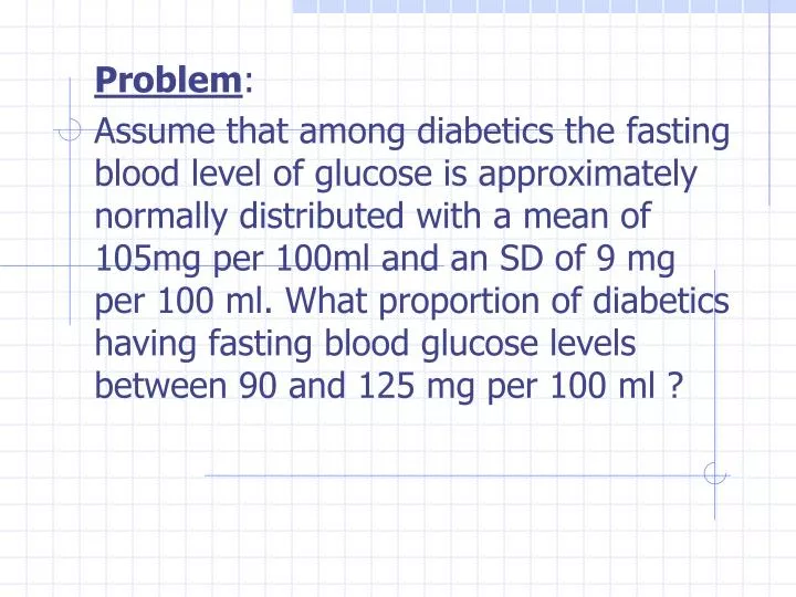
Problem : Assume that among diabetics the fasting blood level of glucose is approximately normally distributed with a mean of 105mg per 100ml and an SD of 9 mg per 100 ml. What proportion of diabetics having fasting blood glucose levels between 90 and 125 mg per 100 ml ?.

E N D
Problem: Assume that among diabetics the fasting blood level of glucose is approximately normally distributed with a mean of 105mg per 100ml and an SD of 9 mg per 100 ml. What proportion of diabetics having fasting blood glucose levels between 90 and 125 mg per 100 ml ?
INTRODUCTION Statistically, a population is the set of all possible values of a variable. Random selection of objects of the population makes the variable a random variable ( it involves chance mechanism) Example: Let ‘x’ be the weight of a newly born baby. ‘x’ is a random variable representing the weight of the baby. The weight of a particular baby is not known until he/she is born.
Discrete random variable: If a random variable can only take values that are whole numbers, it is called a discrete random variable. Example: No. of daily admissions No. of boys in a family of 5 No. of smokers in a group of 100 persons. Continuous random variable: If a random variable can take any value, it is called a continuous random variable. Example: Weight, Height, Age & BP.
Continuous Probability Distributions • Continuous distribution has an infinite number of values between any two values assumed by the continuous variable • As with other probability distributions, the total area under the curve equals 1 • Relative frequency (probability) of occurrence of values between any two points on the x-axis is equal to the total area bounded by the curve, the x-axis, and perpendicular lines erected at the two points on the x-axis
Histogram Figure 1 Histogram of ages of 60 subjects
The Normal or Gaussian distribution is the most important continuous probability distribution in statistics. The term “Gaussian” refers to ‘Carl Freidrich Gauss’ who develop this distribution. The word ‘normal’ here does not mean ‘ordinary’ or ‘common’ nor does it mean ‘disease-free’. It simply means that the distribution conforms to a certain formula and shape.
Histograms • A kind of bar or line chart • Values on the x-axis (horizontal) • Numbers on the y-axis (vertical) • Normal distribution is defined by a particular shape • Symmetrical • Bell-shaped
Gaussian Distribution • Many biologic variables follow this pattern • Hemoglobin, Cholesterol, Serum Electrolytes, Blood pressures, age, weight, height • One can use this information to define what is normal and what is extreme • In clinical medicine 95% or 2 Standard deviations around the mean is normal • Clinically, 5% of “normal” individuals are labeled as extreme/abnormal • We just accept this and move on.
Characteristics of Normal Distribution • Symmetrical about mean, • Mean, median, and mode are equal • Total area under the curve above the x-axis is one square unit • 1 standard deviation on both sides of the mean includes approximately 68% of the total area • 2 standard deviations includes approximately 95% • 3 standard deviations includes approximately 99%
Characteristics of the Normal Distribution • Normal distribution is completely determined by the parameters and • Different values of shift the distribution along the x-axis • Different values of determine degree of flatness or peakedness of the graph
Applications of Normal Distribution • Frequently, data are normally distributed • Essential for some statistical procedures • If not, possible to transform to a more normal form • Approximations for other distributions • Because of the frequent occurrence of the normal distribution in nature, much statistical theory has been developed for it.
What’s so Great about the Normal Distribution? • If you know two things, you know everything about the distribution • Mean • Standard deviation • You know the probability of any value arising
Standardised Scores • My diastolic blood pressure is 100 • So what ? • Normal is 90 (for my age and sex) • Mine is high • But how much high? • Express it in standardised scores • How many SDs above the mean is that?
Mean = 90, SD = 4 (my age and sex) • This is a standardised score, or z-score • Can consult tables (or computer) • See how often this high (or higher) score occur • 99.38% of people have lower scores
Standard Scores • The Z score makes it possible, under some circumstances, to compare scores that originally had different units of measurement.
Z score • Allows you to describe a particular score in terms of where it fits into the overall group of scores. • Whether it is above or below the average and how much it is above or below the average. • A standard score that states the position of a score in relation to the mean of the distribution, using the standard deviation as the unit of measurement. • The number of standard deviations a score is above or below a mean.
Z Score • Suppose you scored a 60 on a numerical test and a 30 on a verbal test. On which test did you perform better? • First, we need to know how other people did on the same tests. • Suppose that the mean score on the numerical test was 50 and the mean score on the verbal test was 20. • You scored 10 points above the mean on each test. • Can you conclude that you did equally well on both tests? • You do not know, because you do not know if 10 points on the numerical test is the same as 10 points on the verbal test.
Z Score • Suppose you scored a 60 on a numerical test and a 30 on a verbal test. On which test did you perform better? • Suppose also that the standard deviation on the numerical test was 15 and the standard deviation on the verbal test was 5. • Now can you determine on which test you did better?
Z score • To find out how many standard deviations away from the mean a particular score is, use the Z formula: Population: Sample:
Z Score In relation to the rest of the people who took the tests, you did better on the verbal test than the numerical test.
Properties of Z scores • The standard deviation of any distribution expressed in Z scores is always one. • In calculating Z scores, the standard deviation of the raw scores is the unit of measurement.
Properties of Z scores • Transforming raw scores to Z scores changes the mean to 0 and the standard deviation to 1, but it does not change the shape of the distribution. • For each raw score we first subtract a constant (the mean) and then divide by a constant (the standard deviation). • The proportional relation that exists among the distances between the scores remains the same. • If the shape of the distribution was not normal before it was transformed, it will not be normal afterward.
The Standard Normal Table • Using the standard normal table, you can find the area under the curve that corresponds with certain scores. • The area under the curve is proportional to the frequency of scores. • The area under the curve gives the probability of that score occurring.
Finding the proportion of observations between the mean and a score when Z = 1.80 Reading the Z Table
Finding the proportion of observations above a score when Z = 1.80 Reading the Z Table
Finding the proportion of observations between a score and the mean when Z = -2.10 Reading the Z Table
Finding the proportion of observations below a score when Z = -2.10 Reading the Z Table
Z scores and the Normal Distribution • Can answer a wide variety of questions about any normal distribution with a known mean and standard deviation. • Will address how to solve two main types of normal curve problems: • Finding a proportion given a score. • Finding a score given a proportion.
Example: Finding a Proportion Below the Mean 1. 2. Use C’ Column 3.
Example: Finding a Proportion Below the Mean 4. 1. 2. Use C’ Column 15.87 % of customers 3.
Example: Finding a Proportion Between the Mean and a Score 3. 1. 2. Use B Column
Example: Finding a Proportion Between the Mean and a Score 4. 1. 2. Use B Column 3. 34.13% of the population
Example: Finding a Proportion Below a Score Given that IQ is normally distributed with a mean of 100 and a standard deviation of 16, what proportion of the population has an IQ below 124? 3. 1. 2. 0.50 + B Column
Example: Finding a Proportion Below a Score Given that IQ is normally distributed with a mean of 100 and a standard deviation of 16, what proportion of the population has an IQ below 124? 4. 1. .50 + .4332 = .9332 .9332 of the population 2. 0.50 + B Column 3.
Example: Finding a Proportion Between Two Scores 3. 1. 2. B’ + B
Example: Finding a Proportion Between Two Scores 1. 4. .4878+.4970=.9848 98.48% 2. B’ + B 3.
Example: Finding a Proportion Between Two Scores Given that scores on the Social Adjustment Scale are normally distributed with a mean of 50 and a standard deviation of 10, what proportion of scores are between 30 and 40? 1. 3. 30 40 2. Larger C’-Smaller C’
Example: Finding a Proportion Between Two Scores 4. Given that scores on the Social Adjustment Scale are normally distributed with a mean of 50 and a standard deviation of 10, what proportion of scores are between 30 and 40? .1587-.0228 =.1359 1. 30 40 2. Larger C’-Smaller C’ 3.
Example: Finding a Score from a Proportion (or Percentile Rank) 3. Given that scores on the Social Adjustment Scale are normally distributed with a mean of 50 and a standard deviation of 10, what two scores correspond to the middle 95%? 1. 4. 2. 0.025 in C and C’