Download
1 / 34
370 likes | 700 Vues
7. Channel Models. 2. Medium Scale Fading : due to shadowing and obstacles. 3. Small Scale Fading : due to multipath. 1. Large Scale Fading : due to distance. Signal Losses due to three Effects:. Wireless Channel.

E N D
2. Medium Scale Fading: due to shadowing and obstacles 3. Small Scale Fading: due to multipath 1. Large Scale Fading: due to distance Signal Losses due to three Effects:
Wireless Channel Frequencies of Interest: in the UHF (.3GHz – 3GHz) and SHF (3GHz – 30 GHz) bands; • Several Effects: • Path Loss due to dissipation of energy: it depends on distance only • Shadowing due to obstacles such as buildings, trees, walls. Is caused by absorption, reflection, scattering … • Self-Interference due to Multipath.
1.1. Large Scale Fading: Free Space Path Loss due to Free Space Propagation: For isotropic antennas: Transmit antenna Receive antenna wavelength Path Loss in dB:
2. Medium Scale Fading: Losses due to Buildings, Trees, Hills, Walls … The Power Loss in dB is random: expected value random, zero mean approximately gaussian with
Values for Exponent : Free Space 2 Urban 2.7-3.5 Indoors (LOS) 1.6-1.8 Indoors(NLOS) 4-6 Average Loss Free space loss at reference distance dB • Reference distance • indoor 1-10m • outdoor 10-100m Path loss exponent
Empirical Models for Propagation Losses to Environment • Okumura: urban macrocells 1-100km, frequencies 0.15-1.5GHz, BS antenna 30-100m high; • Hata: similar to Okumura, but simplified • COST 231: Hata model extended by European study to 2GHz
3. Small Scale Fading due to Multipath. a. Spreading in Time: different paths have different lengths; Receive Transmit time Example for 100m path difference we have a time delay
b. Spreading in Frequency: motion causes frequency shift (Doppler) Receive Transmit time time for each path Doppler Shift Frequency (Hz)
Put everything together Transmit Receive time time
Re{.} LPF LPF channel Each path has … …shift in time … … attenuation… paths …shift in frequency … (this causes small scale time variations)
2.1 Statistical Models of Fading Channels Several Reflectors: Transmit
average time delay • each time delay • each doppler shift For each path with NO Line Of Sight (NOLOS):
Some mathematical manipulation … Assume: bandwidth of signal << … leading to this: with random, time varying
Statistical Model for the time varying coefficients random By the CLT is gaussian, zero mean, with: with the Doppler frequency shift.
Each coefficient is complex, gaussian, WSS with autocorrelation and PSD with maximum Doppler frequency. This is called Jakes spectrum.
Bottom Line. This: time time time … can be modeled as: time time delays
For each path • unit power • time varying (from autocorrelation) • time invariant • from power distribution
Parameters for a Multipath Channel (No Line of Sight): Time delays: sec dB Power Attenuations: Hz Doppler Shift: Summary of Channel Model: WSS with Jakes PSD
Non Line of Sight (NOLOS) and Line of Sight (LOS) Fading Channels • Rayleigh (No Line of Sight). • Specified by: Time delays Power distribution Maximum Doppler 2. Ricean (Line of Sight) Same as Rayleigh, plus Ricean Factor Power through LOS Power through NOLOS
Simulink Example M-QAM Modulation Rayleigh Fading Channel Parameters Bit Rate
Set Numerical Values: modulation power channel velocity carrier freq. Recall the Doppler Frequency: Easy to show that:
Channel Parameterization • Time Spread and Frequency Coherence Bandwidth • Flat Fading vs Frequency Selective Fading • Doppler Frequency Spread and Time Coherence • Slow Fading vs Fast Fading
1. Time Spread and Frequency Coherence Bandwidth transmitted Try a number ofexperiments transmitting a narrow pulse at different random times We obtain a number of received pulses
Received Power time Take theaverage received powerat time More realistically:
This defines the Coherence Bandwidth. Take a complex exponential signal with frequency . The response of the channel is: If then i.e. the attenuation is not frequency dependent Define the Frequency Coherence Bandwidth as
This means that the frequency response of the channel is “flat” within the coherence bandwidth: Channel “Flat” up to the Coherence Bandwidth frequency Coherence Bandwidth Flat Fading Just attenuation, no distortion < Signal Bandwidth Frequency Coherence > Frequency Selective Fading Distortion!!!
Example: Flat Fading Channel : Delays T=[0 10e-6 15e-6] sec Power P=[0, -3, -8] dB Symbol Rate Fs=10kHz Doppler Fd=0.1Hz Modulation QPSK Very low Inter Symbol Interference (ISI) Spectrum: fairly uniform
Example: Frequency Selective Fading Channel : Delays T=[0 10e-6 15e-6] sec Power P=[0, -3, -8] dB Symbol Rate Fs=1MHz Doppler Fd=0.1Hz Modulation QPSK Very high ISI Spectrum with deep variations
transmitted 3. Doppler Frequency Spread and Time Coherence Back to the experiment of sending pulses. Take autocorrelations: Where:
Take the FT of each one: This shows how the multipath characteristics change with time. It defines the Time Coherence: Within the Time Coherence the channel can be considered Time Invariant.
Summary of Time/Frequency spread of the channel Frequency Spread Time Coherence Time Spread Frequency Coherence
Stanford University Interim (SUI) Channel Models Extension of Work done at AT&T Wireless and Erceg etal. • Three terrain types: • Category A: Hilly/Moderate to Heavy Tree density; • Category B: Hilly/ Light Tree density or Flat/Moderate to Heavy Tree density • Category C: Flat/Light Tree density Six different Scenarios (SUI-1 – SUI-6). Found in IEEE 802.16.3c-01/29r4, “Channel Models for Wireless Applications,” http://wirelessman.org/tg3/contrib/802163c-01_29r4.pdf V. Erceg etal, “An Empirical Based Path Loss Model for Wireless Channels in Suburban Environments,” IEEE Selected Areas in Communications, Vol 17, no 7, July 1999