Download
1 / 22
220 likes | 373 Vues
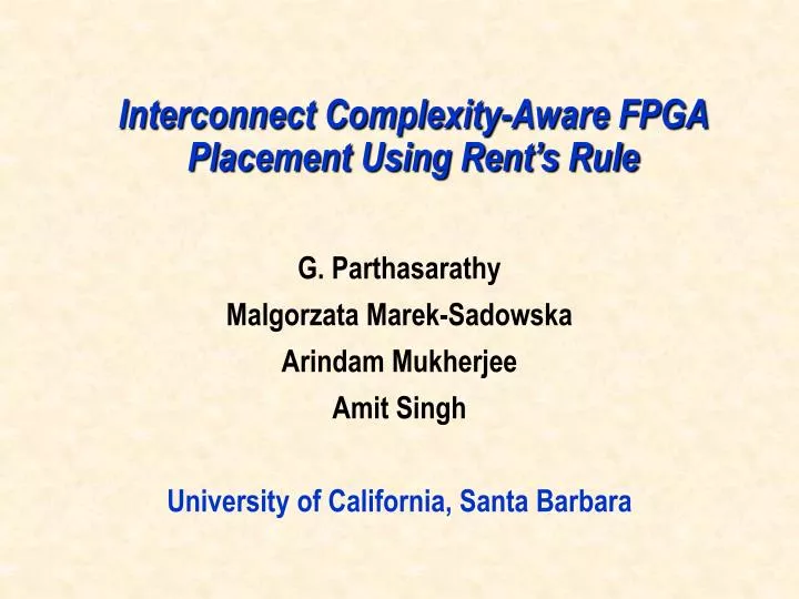
Interconnect Complexity-Aware FPGA Placement Using Rent’s Rule. G. Parthasarathy Malgorzata Marek-Sadowska Arindam Mukherjee Amit Singh University of California, Santa Barbara. Outline. Motivation Rent’s Parameter Analysis New Placement Algorithm Results Conclusions Future Work.

E N D
Interconnect Complexity-Aware FPGA Placement Using Rent’s Rule G. Parthasarathy Malgorzata Marek-Sadowska Arindam Mukherjee Amit Singh University of California, Santa Barbara
Outline • Motivation • Rent’s Parameter • Analysis • New Placement Algorithm • Results • Conclusions • Future Work
Motivation • 80-90% of die area = interconnects • increased programmability • routing resource utilization (RRU) is low • 100% logic utilization • unused LUTs -> better RRU • maybe at the cost of increased area? • Maybe not! • interconnect complexity guided placement - Rent’s parameter
Rent’s Parameter • Common measure for Interconnect Complexity Nio = K NgP Nio – Number of IO pins/terminals external to the logic partition K - Average number of interconnections per LUT Ng – Number of LUTs in a logic partition p – Rent’s parameter after E.F.Rent • E.F.Rent,1960 • Landman, Russo, 1971
Local Rent’s parameter Pld • Complexity Varies across design. • Solution – Use local interconnect complexity measure based in interconnect length distributions. (Van Marck et al.,95) • Reduces to Landman’s Rent’s exponent for uniform design at the top level
Rent’s Parameter • Van Marck, Stroobandt, Campenhout, 1995 • p : D(log Ni) / D(log Li) p – Rent’s parameter Li - length of a net Ni - number of nets of length Li
Analysis • Consists of LUTs, connection boxes and switch-boxes • Regular 2-D mesh array of unit tiles FPGA Architecture
FPGA Fabric Min-Size-Up • Definitions • Pa – Rent’s parameter for Architecture • Pd – Rent’s parameter for Design • Case 1: Pd <= Pa • Design routable. Try to get best placement. • Case 2: Pd > Pa • Design Un-routable. Need more resources. • Solution – Increase FPGA fabric size by scaling factor C Pa = = Pd ) Nio K N K(C.N g g - Pd Pa = C N Pd g
n Bounding_b ox_length( Bi) pld pla ) (1+ - å Track Crossing Function q(i) net = i 1 New Placement Algorithm • Simulated Annealing - VPR • scale-up fabric by C • modify VPR’s existing Cost Function • | pld - pla | used as scaling factor for bounding-box based cost function • uniform distribution of interconnect complexity
placed and routed design pla pld ? > no yes scale-up fabric by C use MVPR Place-and-Route CAD Flow • Generate Benchmarks • Known Pd • Uniform Distribution • Map to Net-list • Place-and-route • VPR • MVPR • Compare
Results - Benchmarks gnl generated ckts p1d = p2d = p3d = p4d = p5d = p6d p6d p5d p4d p1d p2d p3d random ckts - ISCAS benchmarks
Results Rent’s Parameter for Architecture1 • Segmentation = 1, channel width = 7, Pa = 0.62
Rent’s parameter for Architecture2 • Segmentation = 2, channel width = 7, Pa = 0.64
Routing Utilization for seg = 1 • MVPR produces better routing utilization: • 15-25% better
Routing Utilization for seg = 1:2 • MVPR produces better routing utilization: • 10-15% better
Routing Utilization for seg = 2 • MVPR produces only minimally better routing utilization: • 1-5% better
Routing Overhead Results (MVPR vs VPR) seg = 1 • results follow trend for changes in architecture
CLB Area Utilization (MVPR v/s VPR) seg = 1 • results follow trend for changes in architecture • logic area utilization falls with increasing Pd
MVPR over VPR for gnl generated ckts • 25% higher RRU • 10-15% lower Area
MVPR over VPR for ISCAS ckts • same track utilization • 5% lower average wire length • 2-5% higher RRU • 10-15% higher Area
Conclusions • Pluses • New Cost Function • Minimum size fabric derived for Pd > Pa • Min-Area <-> Max-RRU • Minuses • Errors in the estimation of Pd and Pa • second-order effects • Non-uniform interconnect complexities
Future Work • Modifying MVPR • non-uniform interconnect complexity • timing/power-dissipation and complexity-aware FPGA placement • correlating track segmentation with accurate estimation of Rent’s parameter