Download
1 / 70
710 likes | 942 Vues
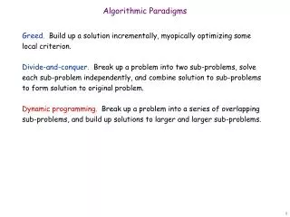
Algorithmic Paradigms. Greed. Build up a solution incrementally, myopically optimizing some local criterion. Divide-and-conquer. Break up a problem into two sub-problems, solve each sub-problem independently, and combine solution to sub-problems to form solution to original problem.

E N D
Algorithmic Paradigms • Greed. Build up a solution incrementally, myopically optimizing some local criterion. • Divide-and-conquer. Break up a problem into two sub-problems, solve each sub-problem independently, and combine solution to sub-problems to form solution to original problem. • Dynamic programming.Break up a problem into a series of overlapping sub-problems, and build up solutions to larger and larger sub-problems.
Dynamic Programming History • Bellman. Pioneered the systematic study of dynamic programming in the 1950s. • Etymology. • Dynamic programming = planning over time. • Secretary of Defense was hostile to mathematical research. • Bellman sought an impressive name to avoid confrontation. • "it's impossible to use dynamic in a pejorative sense" • "something not even a Congressman could object to" Reference: Bellman, R. E. Eye of the Hurricane, An Autobiography.
Dynamic Programming Applications • Areas. • Bioinformatics. • Control theory. • Information theory. • Operations research. • Computer science: theory, graphics, AI, systems, …. • Some famous dynamic programming algorithms. • Viterbi for hidden Markov models. • Unix diff for comparing two files. • Smith-Waterman for sequence alignment. • Bellman-Ford for shortest path routing in networks. • Cocke-Kasami-Younger for parsing context free grammars.
Weighted Interval Scheduling • Weighted interval scheduling problem. • Job j starts at sj, finishes at fj, and has weight or value vj . • Two jobs compatible if they don't overlap. • Goal: find maximum weight subset of mutually compatible jobs. a b c d e f g h Time 0 1 2 3 4 5 6 7 8 9 10 11
Unweighted Interval Scheduling Review • Recall. Greedy algorithm works if all weights are 1. • Consider jobs in ascending order of finish time. • Add job to subset if it is compatible with previously chosen jobs. • Observation. Greedy algorithm can fail spectacularly if arbitrary weights are allowed. weight = 999 b weight = 1 a Time 0 1 2 3 4 5 6 7 8 9 10 11
Weighted Interval Scheduling Notation. Label jobs by finishing time: f1 f2 . . . fn . Def. p(j) = largest index i < j such that job i is compatible with j. Ex: p(8) = 5, p(7) = 3, p(2) = 0. 1 2 3 4 5 6 7 8 Time 0 1 2 3 4 5 6 7 8 9 10 11
Dynamic Programming: Binary Choice • Notation. OPT(j) = value of optimal solution to the problem consisting of job requests 1, 2, ..., j. • Case 1: OPT selects job j. • can't use incompatible jobs { p(j) + 1, p(j) + 2, ..., j - 1 } • must include optimal solution to problem consisting of remaining compatible jobs 1, 2, ..., p(j) • Case 2: OPT does not select job j. • must include optimal solution to problem consisting of remaining compatible jobs 1, 2, ..., j-1 optimal substructure
Weighted Interval Scheduling: Brute Force • Brute force algorithm. Input: n, s1,…,sn , f1,…,fn , v1,…,vn Sort jobs by finish times so that f1 f2 ... fn. Compute p(1), p(2), …, p(n) Compute-Opt(j) { if (j = 0) return 0 else return max(vj + Compute-Opt(p(j)), Compute-Opt(j-1)) }
5 4 3 3 2 2 1 2 1 1 0 1 0 1 0 Weighted Interval Scheduling: Brute Force • Observation. Recursive algorithm fails spectacularly because of redundant sub-problems exponential algorithms. • Ex. Number of recursive calls for family of "layered" instances grows like Fibonacci sequence. 1 2 3 4 5 p(1) = 0, p(j) = j-2
Weighted Interval Scheduling: Memoization • Memoization. Store results of each sub-problem in a cache; lookup as needed. Input: n, s1,…,sn , f1,…,fn , v1,…,vn Sort jobs by finish times so that f1 f2 ... fn. Compute p(1), p(2), …, p(n) forj = 1 to n M[j] = empty M[j] = 0 M-Compute-Opt(j) { if (M[j] is empty) M[j] = max(wj + M-Compute-Opt(p(j)), M-Compute-Opt(j-1)) return M[j] } global array
Weighted Interval Scheduling: Running Time • Claim. Memoized version of algorithm takes O(n log n) time. • Sort by finish time: O(n log n). • Computing p(): O(n) after sorting by start time. • M-Compute-Opt(j): each invocation takes O(1) time and either • (i) returns an existing value M[j] • (ii) fills in one new entry M[j] and makes two recursive calls • Progress measure = # nonempty entries of M[]. • initially = 0, throughout n. • (ii) increases by 1 at most 2n recursive calls. • Overall running time of M-Compute-Opt(n) is O(n). ▪ • Remark. O(n) if jobs are pre-sorted by start and finish times.
F(40) F(39) F(38) F(38) F(37) F(37) F(36) F(37) F(36) F(36) F(35) F(36) F(35) F(35) F(34) Automated Memoization • Automated memoization. Many functional programming languages(e.g., Lisp) have built-in support for memoization. • Q. Why not in imperative languages (e.g., Java)? static int F(int n) { if (n <= 1) return n; else return F(n-1) + F(n-2); } (defun F (n) (if (<= n 1) n (+ (F (- n 1)) (F (- n 2))))) Java (exponential) Lisp (efficient)
Weighted Interval Scheduling: Finding a Solution • Q. Dynamic programming algorithms computes optimal value. What if we want the solution itself? • A. Do some post-processing. • # of recursive calls n O(n). Run M-Compute-Opt(n) Run Find-Solution(n) Find-Solution(j) { if (j = 0) output nothing else if (vj + M[p(j)] > M[j-1]) print j Find-Solution(p(j)) else Find-Solution(j-1) }
Weighted Interval Scheduling: Bottom-Up • Bottom-up dynamic programming. Unwind recursion. Input: n, s1,…,sn , f1,…,fn , v1,…,vn Sort jobs by finish times so that f1 f2 ... fn. Compute p(1), p(2), …, p(n) Iterative-Compute-Opt { M[0] = 0 forj = 1 to n M[j] = max(vj + M[p(j)], M[j-1]) }
Segmented Least Squares • Least squares. • Foundational problem in statistic and numerical analysis. • Given n points in the plane: (x1, y1), (x2, y2) , . . . , (xn, yn). • Find a line y = ax + b that minimizes the sum of the squared error: • Solution. Calculus min error is achieved when y x
Segmented Least Squares • Segmented least squares. • Points lie roughly on a sequence of several line segments. • Given n points in the plane (x1, y1), (x2, y2) , . . . , (xn, yn) with • x1 < x2 < ... < xn, find a sequence of lines that minimizes f(x). • Q. What's a reasonable choice for f(x) to balance accuracy and parsimony? goodness of fit number of lines y x
Segmented Least Squares • Segmented least squares. • Points lie roughly on a sequence of several line segments. • Given n points in the plane (x1, y1), (x2, y2) , . . . , (xn, yn) with • x1 < x2 < ... < xn, find a sequence of lines that minimizes: • the sum of the sums of the squared errors E in each segment • the number of lines L • Tradeoff function: E + c L, for some constant c > 0. y x
Dynamic Programming: Multiway Choice • Notation. • OPT(j) = minimum cost for points p1, pi+1 , . . . , pj. • e(i, j) = minimum sum of squares for points pi, pi+1 , . . . , pj. • To compute OPT(j): • Last segment uses points pi, pi+1 , . . . , pj for some i. • Cost = e(i, j) + c + OPT(i-1).
Segmented Least Squares: Algorithm • Running time. O(n3). • Bottleneck = computing e(i, j) for O(n2) pairs, O(n) per pair using previous formula. INPUT: n, p1,…,pN , c Segmented-Least-Squares() { M[0] = 0 for j = 1 to n for i = 1 to j compute the least square error eij for the segment pi,…, pj for j = 1 to n M[j] = min 1 i j (eij + c + M[i-1]) return M[n] } can be improved to O(n2) by pre-computing various statistics
Knapsack Problem • Knapsack problem. • Given n objects and a "knapsack." • Item i weighs wi > 0 kilograms and has value vi > 0. • Knapsack has capacity of W kilograms. • Goal: fill knapsack so as to maximize total value. • Ex: { 3, 4 } has value 40. • Greedy: repeatedly add item with maximum ratio vi / wi. • Ex: { 5, 2, 1 } achieves only value = 35 greedy not optimal. Item Value Weight 1 1 1 2 6 2 W = 11 3 18 5 4 22 6 5 28 7
Dynamic Programming: False Start • Def. OPT(i) = max profit subset of items 1, …, i. • Case 1: OPT does not select item i. • OPT selects best of { 1, 2, …, i-1 } • Case 2: OPT selects item i. • accepting item i does not immediately imply that we will have to reject other items • without knowing what other items were selected before i, we don't even know if we have enough room for i • Conclusion. Need more sub-problems!
Dynamic Programming: Adding a New Variable • Def. OPT(i, w) = max profit subset of items 1, …, i with weight limit w. • Case 1: OPT does not select item i. • OPT selects best of { 1, 2, …, i-1 } using weight limit w • Case 2: OPT selects item i. • new weight limit = w – wi • OPT selects best of { 1, 2, …, i–1 } using this new weight limit
Knapsack Problem: Bottom-Up • Knapsack. Fill up an n-by-W array. Input: n, w1,…,wN, v1,…,vN for w = 0 to W M[0, w] = 0 for i = 1 to n for w = 1 to W if (wi > w) M[i, w] = M[i-1, w] else M[i, w] = max {M[i-1, w], vi + M[i-1, w-wi ]} return M[n, W]
0 1 2 3 4 5 6 7 8 9 10 11 0 0 0 0 0 0 0 0 0 0 0 0 { 1 } 0 1 1 1 1 1 1 1 1 1 1 1 { 1, 2 } 0 1 6 7 7 7 7 7 7 7 7 7 { 1, 2, 3 } 0 1 6 7 7 18 19 24 25 25 25 25 { 1, 2, 3, 4 } 0 1 6 7 7 18 22 24 28 29 29 40 { 1, 2, 3, 4, 5 } 0 1 6 7 7 18 22 28 29 34 34 40 Item Value Weight 1 1 1 2 6 2 3 18 5 4 22 6 5 28 7 Knapsack Algorithm W + 1 n + 1 OPT: { 4, 3 } value = 22 + 18 = 40 W = 11
Knapsack Problem: Running Time • Running time. (n W). • Not polynomial in input size! • "Pseudo-polynomial." • Decision version of Knapsack is NP-complete. [Chapter 8] • Knapsack approximation algorithm. There exists a polynomial algorithm that produces a feasible solution that has value within 0.01% of optimum. [Section 11.8]
RNA Secondary Structure • RNA. String B = b1b2bn over alphabet { A, C, G, U }. • Secondary structure. RNA is single-stranded so it tends to loop back and form base pairs with itself. This structure is essential for understanding behavior of molecule. C A Ex: GUCGAUUGAGCGAAUGUAACAACGUGGCUACGGCGAGA A A A U G C C G U A A G G U A U U A G A C G C U G C G C G A G C G A U G complementary base pairs: A-U, C-G
RNA Secondary Structure • Secondary structure. A set of pairs S = { (bi, bj) } that satisfy: • [Watson-Crick.] S is a matching and each pair in S is a Watson-Crick complement: A-U, U-A, C-G, or G-C. • [No sharp turns.] The ends of each pair are separated by at least 4 intervening bases. If (bi, bj) S, then i < j - 4. • [Non-crossing.] If (bi, bj) and (bk, bl) are two pairs in S, then we cannot have i < k < j < l. • Free energy. Usual hypothesis is that an RNA molecule will form the secondary structure with the optimum total free energy. • Goal. Given an RNA molecule B = b1b2bn, find a secondary structure S that maximizes the number of base pairs. approximate by number of base pairs
RNA Secondary Structure: Examples • Examples. G G G G G G G C U C U G C G C U C A U A U A G U A U A U A base pair U G U G G C C A U U G G G C A U G U U G G C C A U G A A A 4 ok sharp turn crossing
RNA Secondary Structure: Subproblems • First attempt. OPT(j) = maximum number of base pairs in a secondary structure of the substring b1b2bj. • Difficulty. Results in two sub-problems. • Finding secondary structure in: b1b2bt-1. • Finding secondary structure in: bt+1bt+2bn-1. match bt and bn t n 1 OPT(t-1) need more sub-problems
Dynamic Programming Over Intervals • Notation. OPT(i, j) = maximum number of base pairs in a secondary structure of the substring bibi+1bj. • Case 1. If i j - 4. • OPT(i, j) = 0 by no-sharp turns condition. • Case 2. Base bj is not involved in a pair. • OPT(i, j) = OPT(i, j-1) • Case 3. Base bj pairs with bt for some i t < j - 4. • non-crossing constraint decouples resulting sub-problems • OPT(i, j) = 1 + maxt { OPT(i, t-1) + OPT(t+1, j-1) } • Remark. Same core idea in CKY algorithm to parse context-free grammars. take max over t such that i t < j-4 andbt and bj are Watson-Crick complements
Bottom Up Dynamic Programming Over Intervals • Q. What order to solve the sub-problems? • A. Do shortest intervals first. • Running time. O(n3). RNA(b1,…,bn) { for k = 5, 6, …, n-1 for i = 1, 2, …, n-k j = i + k Compute M[i, j] return M[1, n] } 4 0 0 0 3 0 0 i 0 2 1 6 7 8 9 using recurrence j
Dynamic Programming Summary • Recipe. • Characterize structure of problem. • Recursively define value of optimal solution. • Compute value of optimal solution. • Construct optimal solution from computed information. • Dynamic programming techniques. • Binary choice: weighted interval scheduling. • Multi-way choice: segmented least squares. • Adding a new variable: knapsack. • Dynamic programming over intervals: RNA secondary structure. • Top-down vs. bottom-up: different people have different intuitions. Viterbi algorithm for HMM also usesDP to optimize a maximum likelihoodtradeoff between parsimony and accuracy CKY parsing algorithm for context-freegrammar has similar structure
String Similarity • How similar are two strings? • ocurrance • occurrence o c u r r a n c e - o c c u r r e n c e 5 mismatches, 1 gap o c - u r r a n c e o c c u r r e n c e 1 mismatch, 1 gap o c - u r r - a n c e o c c u r r e - n c e 0 mismatches, 3 gaps
Edit Distance • Applications. • Basis for Unix diff. • Speech recognition. • Computational biology. • Edit distance. [Levenshtein 1966, Needleman-Wunsch 1970] • Gap penalty ; mismatch penalty pq. • Cost = sum of gap and mismatch penalties. C T G A C C T A C C T - C T G A C C T A C C T C C T G A C T A C A T C C T G A C - T A C A T TC + GT + AG+ 2CA 2+ CA
Sequence Alignment • Goal: Given two strings X = x1 x2 . . . xm and Y = y1 y2 . . . yn find alignment of minimum cost. • Def. An alignment M is a set of ordered pairs xi-yj such that each item occurs in at most one pair and no crossings. • Def. The pair xi-yj and xi'-yj'cross if i < i', but j > j'. • Ex:CTACCG vs. TACATG.Sol: M = x2-y1, x3-y2, x4-y3, x5-y4, x6-y6. x1 x2 x3 x4 x5 x6 C T A C C - G - T A C A T G y1 y2 y3 y4 y5 y6
Sequence Alignment: Problem Structure • Def. OPT(i, j) = min cost of aligning strings x1 x2 . . . xi and y1 y2 . . . yj. • Case 1: OPT matches xi-yj. • pay mismatch for xi-yj + min cost of aligning two stringsx1 x2 . . . xi-1 and y1 y2 . . . yj-1 • Case 2a: OPT leaves xi unmatched. • pay gap for xi and min cost of aligning x1 x2 . . . xi-1 and y1 y2 . . . yj • Case 2b: OPT leaves yj unmatched. • pay gap for yj and min cost of aligning x1 x2 . . . xi and y1 y2 . . . yj-1
Sequence Alignment: Algorithm • Analysis. (mn) time and space. • English words or sentences: m, n 10. • Computational biology: m = n = 100,000. 10 billions ops OK, but 10GB array? Sequence-Alignment(m, n, x1x2...xm, y1y2...yn, , ) { for i = 0 to m M[0, i] = i for j = 0 to n M[j, 0] = j for i = 1 to m for j = 1 to n M[i, j] = min([xi, yj] + M[i-1, j-1], + M[i-1, j], + M[i, j-1]) return M[m, n] }
Sequence Alignment: Linear Space • Q. Can we avoid using quadratic space? • Easy. Optimal value in O(m + n) space and O(mn) time. • Compute OPT(i, •) from OPT(i-1, •). • No longer a simple way to recover alignment itself. • Theorem. [Hirschberg 1975]Optimal alignment in O(m + n) space and O(mn) time. • Clever combination of divide-and-conquer and dynamic programming. • Inspired by idea of Savitch from complexity theory.
Sequence Alignment: Linear Space • Edit distance graph. • Let f(i, j) be shortest path from (0,0) to (i, j). • Observation: f(i, j) = OPT(i, j). y1 y2 y3 y4 y5 y6 0-0 x1 i-j x2 m-n x3
Sequence Alignment: Linear Space • Edit distance graph. • Let f(i, j) be shortest path from (0,0) to (i, j). • Can compute f (•, j) for any j in O(mn) time and O(m + n) space. j y1 y2 y3 y4 y5 y6 0-0 x1 i-j x2 m-n x3
Sequence Alignment: Linear Space • Edit distance graph. • Let g(i, j) be shortest path from (i, j) to (m, n). • Can compute by reversing the edge orientations and inverting the roles of (0, 0) and (m, n) y1 y2 y3 y4 y5 y6 0-0 i-j x1 x2 m-n x3
Sequence Alignment: Linear Space • Edit distance graph. • Let g(i, j) be shortest path from (i, j) to (m, n). • Can compute g(•, j) for any j in O(mn) time and O(m + n) space. j y1 y2 y3 y4 y5 y6 0-0 i-j x1 x2 m-n x3
Sequence Alignment: Linear Space • Observation 1. The cost of the shortest path that uses (i, j) isf(i, j) + g(i, j). y1 y2 y3 y4 y5 y6 0-0 i-j x1 x2 m-n x3
Sequence Alignment: Linear Space • Observation 2. let q be an index that minimizes f(q, n/2) + g(q, n/2). Then, the shortest path from (0, 0) to (m, n) uses (q, n/2). n / 2 y1 y2 y3 y4 y5 y6 0-0 q i-j x1 x2 m-n x3